Integración Monte Carlo en Python

La integración de Monte Carlo es un proceso de resolución de integrales que tiene numerosos valores para integrar. El proceso de Monte Carlo utiliza la teoría de los grandes números y el muestreo aleatorio para aproximar valores que están muy cerca de la solución real de la integral. Funciona en el promedio de una función denotada por <f(x)> . Luego podemos expandir <f(x)> como la suma de los valores divididos por el número de puntos en la integración y resolver el lado izquierdo de la ecuación para aproximar el valor de la integración en el lado derecho. La derivación es la siguiente.

Donde N = no. de términos utilizados para la aproximación de los valores.

Ahora, primero calcularíamos la integral utilizando el método de Monte Carlo numéricamente y luego, finalmente, visualizaríamos el resultado utilizando un histograma utilizando la biblioteca de python matplotlib.

Módulos utilizados:

Los módulos que se utilizarían son:

• Scipy : se utiliza para obtener valores aleatorios entre los límites de la integral. Se puede instalar usando:

pip install scipy # for windows
or
pip3 install scipy # for linux and macos

• Numpy : se utiliza para formar arrays y almacenar diferentes valores. Se puede instalar usando:

pip install numpy # for windows
or 
pip3 install numpy # for linux and macos

• Matplotlib : Se utiliza para visualizar el histograma y el resultado de la integración de Monte Carlo.

pip install matplotlib # for windows
or 
pip3 install matplotlib # for linux and macos

Ejemplo 1:

La integral que vamos a evaluar es:

Una vez que hayamos terminado de instalar los módulos, ahora podemos comenzar a escribir código importando los módulos necesarios, scipy para crear valores aleatorios en un rango y el módulo NumPy para crear arrays estáticas, ya que las listas predeterminadas en python son relativamente lentas debido a la asignación de memoria dinámica. Luego definimos los límites de integración que son 0 y pi (usamos np.pi para obtener el valor de pi. Luego creamos una array numpy estática de ceros de tamaño N usando np. zeros(N). Ahora iteramos sobre cada índice de la array N y lo llenamos con valores aleatorios entre a y b. Luego creamos una variable para almacenar la suma de las funciones de diferentes valores de la variable integral. Ahora creamos una función para calcular el seno de un valor particular de x Luego iteramos y sumamos todos los valores devueltos por la función de x para diferentes valores de x a la integral variable. Luego usamos la fórmula derivada arriba para obtener los resultados. Finalmente, imprimimos los resultados en la línea final.

# importing the modules
from scipy import random
import numpy as np
  
# limits of integration
a = 0
b = np.pi # gets the value of pi
N = 1000
  
# array of zeros of length N
ar = np.zeros(N)
  
# iterating over each Value of ar and filling 
# it with a random value between the limits a
# and b
for i in range (len(ar)):
    ar[i] = random.uniform(a,b)
  
# variable to store sum of the functions of 
# different values of x
integral = 0.0
  
# function to calculate the sin of a particular
# value of x
def f(x):
    return np.sin(x)
  
# iterates and sums up values of different functions
# of x
for i in ar:
    integral += f(i)
  
# we get the answer by the formula derived adobe
ans = (b-a)/float(N)*integral
  
# prints the solution
print ("The value calculated by monte carlo integration is {}.".format(ans))

Producción:

El valor calculado por la integración de monte carlo es 2.0256756150767035.

El valor obtenido es muy cercano a la respuesta real de la integral que es 2.0. 

Ahora, si queremos visualizar la integración usando un histograma, podemos hacerlo usando la biblioteca matplotlib. Nuevamente importamos los módulos, definimos los límites de integración y escribimos la función sin para calcular el valor sin para un valor particular de x. Luego, tomamos una array que tiene variables que representan cada haz del histograma. Luego iteramos a través de N valores y repetimos el mismo proceso de crear una array de ceros, llenándola con valores x aleatorios, creando una variable integral sumando todos los valores de la función y obteniendo la respuesta N veces, cada respuesta representando un haz del histograma . El código es el siguiente:

# importing the modules
from scipy import random
import numpy as np
import matplotlib.pyplot as plt
  
# limits of integration
a = 0
b = np.pi # gets the value of pi
N = 1000
  
# function to calculate the sin of a particular 
# value of x
def f(x):
    return np.sin(x)
  
# list to store all the values for plotting 
plt_vals = []
  
# we iterate through all the values to generate 
# multiple results and show whose intensity is 
# the most.
for i in range(N):
    
    #array of zeros of length N
    ar = np.zeros(N)
  
    # iterating over each Value of ar and filling it
    # with a random value between the limits a and b
    for i in range (len(ar)):
        ar[i] = random.uniform(a,b)
  
    # variable to store sum of the functions of different
    # values of x
    integral = 0.0
  
    # iterates and sums up values of different functions 
    # of x
    for i in ar:
        integral += f(i)
  
    # we get the answer by the formula derived adobe
    ans = (b-a)/float(N)*integral
  
    # appends the solution to a list for plotting the graph
    plt_vals.append(ans)
  
# details of the plot to be generated
# sets the title of the plot 
plt.title("Distributions of areas calculated")
  
# 3 parameters (array on which histogram needs 
plt.hist (plt_vals, bins=30, ec="black") 
  
# to be made, bins, separators colour between the
# beams)
# sets the label of the x-axis of the plot
plt.xlabel("Areas")
plt.show() # shows the plot

Producción:

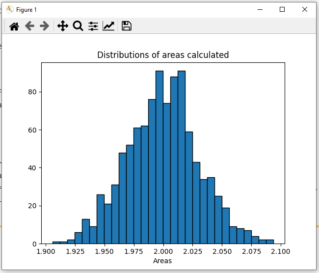
Aquí, como podemos ver, los resultados más probables de acuerdo con este gráfico serían 2,023 o 2,024, que nuevamente está bastante cerca de la solución real de esta integral que es 2,0.  

Ejemplo 2:

La integral que vamos a evaluar es: 

La implementación sería la misma que la pregunta anterior, solo cambiarían los límites de integración definidos por a y b y también la función f(x) que devuelve el valor de función correspondiente a un valor específico ahora devolvería x^2 en lugar de sin (X). El código para esto sería: 

# importing the modules
from scipy import random
import numpy as np
  
# limits of integration
a = 0
b = 1
N = 1000
  
# array of zeros of length N
ar = np.zeros(N)
  
# iterating over each Value of ar and filling
# it with a random value between the limits a 
# and b
for i in range(len(ar)):
    ar[i] = random.uniform(a, b)
  
# variable to store sum of the functions of 
# different values of x
integral = 0.0
  
# function to calculate the sin of a particular 
# value of x
def f(x):
    return x**2
  
# iterates and sums up values of different 
# functions of x
for i in ar:
    integral += f(i)
  
# we get the answer by the formula derived adobe
ans = (b-a)/float(N)*integral
  
# prints the solution
print("The value calculated by monte carlo integration is {}.".format(ans))

Producción:

El valor calculado por la integración de monte carlo es 0.33024026610116575.

El valor obtenido es muy cercano a la respuesta real de la integral que es 0.333.

Ahora, si queremos visualizar la integración usando un histograma nuevamente, podemos hacerlo usando la biblioteca matplotlib como lo hicimos para el anterior, en este caso, las funciones f (x) devuelven x ^ 2 en lugar de sin (x), y los límites de integración cambian de 0 a 1. El código es el siguiente:

# importing the modules
from scipy import random
import numpy as np
import matplotlib.pyplot as plt
  
# limits of integration
a = 0
b = 1
N = 1000
  
# function to calculate x^2 of a particular value 
# of x
def f(x):
    return x**2
  
# list to store all the values for plotting 
plt_vals = []
  
# we iterate through all the values to generate
# multiple results and show whose intensity is 
# the most. 
for i in range(N):
    
    # array of zeros of length N
    ar = np.zeros(N)
  
    # iterating over each Value of ar and filling
    # it with a random value between the limits a 
    # and b
    for i in range (len(ar)):
        ar[i] = random.uniform(a,b)
  
    # variable to store sum of the functions of 
    # different values of x
    integral = 0.0
  
    # iterates and sums up values of different functions
    # of x
    for i in ar:
        integral += f(i)
  
    # we get the answer by the formula derived adobe
    ans = (b-a)/float(N)*integral
  
    # appends the solution to a list for plotting the 
    # graph
    plt_vals.append(ans)
  
# details of the plot to be generated
# sets the title of the plot 
plt.title("Distributions of areas calculated")
  
# 3 parameters (array on which histogram needs 
# to be made, bins, separators colour between 
# the beams)
plt.hist (plt_vals, bins=30, ec="black")
  
# sets the label of the x-axis of the plot
plt.xlabel("Areas")
plt.show() # shows the plot

Producción:

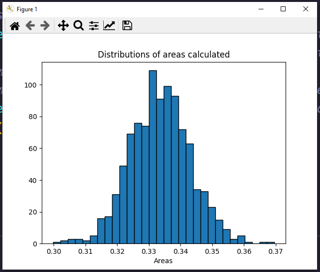
Aquí como podemos ver, los resultados más probables según esta gráfica serían 0.33 que es casi igual (igual en este caso, pero generalmente no ocurre) a la solución real de esta integral que es 0.333.