En este artículo, veremos cómo cargar y jugar con los datos dentro de arrays y vectores en Octave. Aquí hay algunos comandos básicos y funciones relacionadas con arrays y vectores en Octave:
1. Las dimensiones de la array: Podemos encontrar las dimensiones de una array o vector usando la size()función.
% declaring the matrix
M = [1 2 3; 4 5 6; 7 8 9];

% dimensions of the matrix
size(M)

% number of rows
rows = size(M, 1)

% number of columns
cols = size(M, 2)
Producción :
ans =

   3   3

rows =  3
cols =  3
2. Acceder a los elementos de la array: Se puede acceder a los elementos de una array pasando la ubicación del elemento entre paréntesis. En Octave, la indexación comienza desde 1.
% declaring the matrix
M = [1 2 3; 4 5 6; 7 8 9];

% accessing the element at index (2, 3)
% i.e. 2nd row and 3rd column
M(2, 3)

% print the 3rd row
M(3, : )

% print the 1st column
M(:, 1)

% print every thing from 1st and 3rd row
M([1, 3], : )
Producción :
ans =  6

ans =

   7   8   9

ans =

   1
   4
   7

ans =

   1   2   3
   7   8   9
3. Dimensión más larga:length() la función devuelve el tamaño de la dimensión más larga de la array/vector.
% declaring the row vector
M1 = [1 2 3 4 5 6 7 8 9 10];
len_M1 = length(M1)

% declaring the matrix
M2 = [1 2 3; 4 5 6];
len_M2 = length(M2)
Producción :
len_M1 =  10
len_M2 =  3
4. Carga de datos: Primero que nada, veamos cómo identificar los directorios en Octave:
% see the present working directory
pwd

% see the directory's of the folder in which you are
ls
Producción :
ans = /home/dikshant
derby.log  Desktop  Documents  Downloads  Music  Pictures  Public  ${system:java.io.tmpdir}  Templates  Videos
Ahora, antes de cargar los datos, debemos cambiar nuestro directorio de trabajo actual a la ubicación donde se almacenan nuestros datos. Podemos hacer esto con el cdcomando y luego cargarlo de la siguiente manera:
% changing the directory
cd /home/dikshant/Documents/Octave-Project

% list the data present in this directory
ls
Producción :
Feature.dat target.dat
Aquí hemos tomado los datos de las puntuaciones de un alumno como Característica y sus notas como variable objetivo.
Este es el archivo Feature.dat que consta de 25 registros de las horas de estudio de los estudiantes.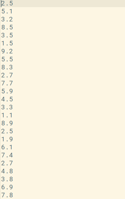
Este es el archivo target.dat que consta de 25 registros de calificaciones de los estudiantes.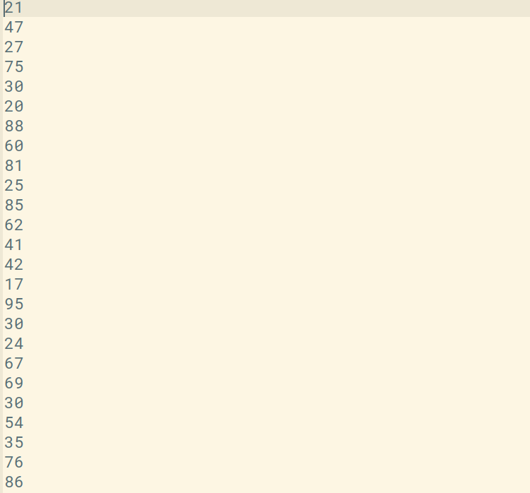
Podemos cargar el archivo con el loadcomando en Octave, en realidad hay 2 formas de cargar los datos, ya sea simplemente con el comando de carga o usando el nombre del archivo como una string en load(). Podemos usar el nombre del archivo como Featureo targetpara imprimir sus datos.
% loading Feature.dat
load Feature.dat % or load('Feature.dat')

% loading target.dat
load target.dat  % or load('target.dat')

% print Feature data
Feature

% print target data
target

% displaying the size of Feature file i.e. the number of data records and column
Feature_size = size(Feature)

% displaying the size of target file i.e. the number of data records and column
target_size = size(target)
Producción :
Feature =

   2.5000
   5.1000
   3.2000
   8.5000
   3.5000
   1.5000
   9.2000
   5.5000
   8.3000
   2.7000
   7.7000
   5.9000
   4.5000
   3.3000
   1.1000
   8.9000
   2.5000
   1.9000
   6.1000
   7.4000
   2.7000
   4.8000
   3.8000
   6.9000
   7.8000

target =

   21
   47
   27
   75
   30
   20
   88
   60
   81
   25
   85
   62
   41
   42
   17
   95
   30
   24
   67
   69
   30
   54
   35
   76
   86

Feature_size =

   25    1

target_size =

   25    1
Podemos usar whoel comando para conocer las variables en nuestro ámbito de octava actual o whospara obtener una descripción más detallada.
% using the who command
who

% using the whos command
whos
Producción:
Variables in the current scope:

Feature  M        M1       M2       ans      target

Variables in the current scope:

   Attr Name         Size                     Bytes  Class
   ==== ====         ====                     =====  =====
        Feature     25x1                        200  double
        M            3x3                         72  double
        M1           1x10                        80  double
        M2           2x3                         48  double
        ans          1x2                         16  double
        target      25x1                        200  double

Total is 77 elements using 616 bytes
También podemos seleccionar algunas de las filas de un archivo cargado, por ejemplo, en nuestro caso, los datos de 25 registros están presentes en la función y el objetivo, podemos crear alguna otra variable para almacenar las filas de datos recortadas como se muestra a continuación:
% storing initial 5 records of Feature in var
var = Feature(1:5)

% storing initial 5 records of target in var1
var1 = target(1:5)

% saving the data of var in a file named modified_Feature.mat in binary format
modified_Feature.mat in binary format

% saving the data of var1 in a file named modified_target.mat in binary format
modified_target.mat in binary format

% saves the data in a readable format
save Feature_data.txt var -ASCII
Producción:
var =

   2.5000
   5.1000
   3.2000
   8.5000
   3.5000

var1 =

   21
   47
   27
   75
   30
5. Modificación de datos: Veamos ahora cómo modificar los datos de arrays y vectores.
% declaring the matrix
M = [1 2 3; 4 5 6; 7 8 9];

% modifying the data of 2nd column for each entry
M(:, 2) = [54; 56; 98]

% declaring the matrix
m = [0 0 0; 0 0 0; 0 0 0];

% modifying the data of 3nd row for each entry
m(3, 🙂 = [100; 568; 987]
Producción :
M =

    1   54    3
    4   56    6
    7   98    9

m =

     0     0     0
     0     0     0
   100   568   987
También podemos agregar las nuevas columnas y filas en una array existente:
% declaring the matrix
M = [1 2 3; 4 5 6; 7 8 9];

% appending the new column vector to your matrix
M = [M, [20;30;40]];

% putting all values of matrix M in a single column vector
M(:)
Producción :
ans =

    1
    4
    7
    2
    5
    8
    3
    6
    9
   20
   30
   40
También podemos concatenar 2 arrays diferentes:
% declaring the matrices
a = [10 20; 30 40; 50 60];
b = [11 22; 33 44; 55 66];

% concatenate matrix as "a" on the left and "b" on the right
c = [a b]

% concatenate matrix as "a" on the top and "b" on the bottom
c = [a ; b]
Producción :
c =

   10   20   11   22
   30   40   33   44
   50   60   55   66

c =

   10   20
   30   40
   50   60
   11   22
   33   44
   55   66
Publicación traducida automáticamente
Artículo escrito por dikshantmalidev y traducido por Barcelona Geeks. The original can be accessed here. Licence: CCBY-SA