IIR significa Infinite Impulse Response. Es una de las características sorprendentes de muchos sistemas invariantes en el tiempo lineal que se distinguen por tener una respuesta de impulso h(t)/h(n) que no se vuelve cero después de algún punto sino que continúa infinitamente. .
¿Qué es el filtro IIR Chebyshev?
IIR Chebyshev es un filtro que es invariable en el tiempo lineal al igual que Butterworth, sin embargo, tiene una caída más pronunciada en comparación con el filtro Butterworth. El filtro Chebyshev se clasifica además como Chebyshev Tipo-I y Chebyshev Tipo-II de acuerdo con parámetros como la ondulación de banda de paso y la ondulación de parada.
¿En qué se diferencia el filtro Chebyshev de Butterworth?
El filtro Chebyshev tiene una caída más pronunciada en comparación con el filtro Butterworth.
¿Qué es el filtro tipo I de Chebyshev?
Chebyshev Type-I minimiza la diferencia absoluta entre la respuesta de frecuencia ideal y real en toda la banda de paso al incorporar una ondulación igual en la banda de paso.
Las especificaciones son las siguientes:
- Frecuencia de banda de paso: 1400-2100 Hz
- Frecuencia de banda de parada: 1050-24500 Hz
- Ondulación de banda de paso: 0.4dB
- Atenuación de la banda de parada: 50 dB
- Frecuencia de muestreo: 7 kHz
Graficaremos la magnitud, fase, impulso, respuesta de paso del filtro.
Enfoque paso a paso:
Paso 1: Importación de todas las bibliotecas necesarias.
Python3
import numpy as np
import scipy.signal as signal
import matplotlib.pyplot as plt
Paso 2: Definición de las funciones definidas por el usuario, como mfreqz() e impz().
Python3
def mfreqz(b, a, Fs):

    # Compute frequency response of the filter
    # using signal.freqz function
    wz, hz = signal.freqz(b, a)

    # Calculate Magnitude from hz in dB
    Mag = 20*np.log10(abs(hz))

    # Calculate phase angle in degree from hz
    Phase = np.unwrap(np.arctan2(np.imag(hz), np.real(hz)))*(180/np.pi)

    # Calculate frequency in Hz from wz
    Freq = wz*Fs/(2*np.pi)

    # Plot filter magnitude and phase responses using subplot.
    fig = plt.figure(figsize=(10, 6))

    # Plot Magnitude response
    sub1 = plt.subplot(2, 1, 1)
    sub1.plot(Freq, Mag, 'r', linewidth=2)
    sub1.axis([1, Fs/2, -100, 5])
    sub1.set_title('Magnitude Response', fontsize=20)
    sub1.set_xlabel('Frequency [Hz]', fontsize=20)
    sub1.set_ylabel('Magnitude [dB]', fontsize=20)
    sub1.grid()

    # Plot phase angle
    sub2 = plt.subplot(2, 1, 2)
    sub2.plot(Freq, Phase, 'g', linewidth=2)
    sub2.set_ylabel('Phase (degree)', fontsize=20)
    sub2.set_xlabel(r'Frequency (Hz)', fontsize=20)
    sub2.set_title(r'Phase response', fontsize=20)
    sub2.grid()

    plt.subplots_adjust(hspace=0.5)
    fig.tight_layout()
    plt.show()

# Define impz(b,a) to calculate impulse response
# and step response of a system
# input: b= an array containing numerator coefficients,
#a= an array containing denominator coefficients
def impz(b, a):

    # Define the impulse sequence of length 60
    impulse = np.repeat(0., 60)
    impulse[0] = 1.
    x = np.arange(0, 60)

    # Compute the impulse response
    response = signal.lfilter(b, a, impulse)

    # Plot filter impulse and step response:
    fig = plt.figure(figsize=(10, 6))
    plt.subplot(211)
    plt.stem(x, response, 'm', use_line_collection=True)
    plt.ylabel('Amplitude', fontsize=15)
    plt.xlabel(r'n (samples)', fontsize=15)
    plt.title(r'Impulse response', fontsize=15)

    plt.subplot(212)
    step = np.cumsum(response)

    # Compute step response of the system
    plt.stem(x, step, 'g', use_line_collection=True)
    plt.ylabel('Amplitude', fontsize=15)
    plt.xlabel(r'n (samples)', fontsize=15)
    plt.title(r'Step response', fontsize=15)
    plt.subplots_adjust(hspace=0.5)

    fig.tight_layout()
    plt.show()
Paso 3: Definir variables con las especificaciones dadas del filtro.
Python3
# Given specification
Fs = 7000  # Sampling frequency in Hz
fp = np.array([1400, 2100])  # Pass band frequency in Hz
fs = np.array([1050, 2450])  # Stop band frequency in Hz
Ap = 0.4  # Pass band ripple in dB
As = 50  # stop band attenuation in dB
Paso 4: Cálculo de la frecuencia de corte
Python3
# Compute pass band and stop band edge frequencies
wp = fp/(Fs/2)  # Normalized passband edge frequencies w.r.t. Nyquist rate
ws = fs/(Fs/2)  # Normalized stopband edge frequencies
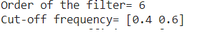
Paso 5: Calcular la frecuencia de corte y el orden
Python3
# Compute order of the  Chebyshev type-1 filter using signal.cheb1ord
N, wc = signal.cheb1ord(wp, ws, Ap, As)

# Print the order of the filter and cutoff frequencies
print('Order of the filter=', N)
print('Cut-off frequency=', wc)
Producción:
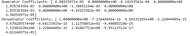
Paso 6: Calcule el coeficiente de filtro
Python
# Design digital Chebyshev type-1 filter
# using signal.cheby1 function
z, p = signal.cheby1(N, Ap, wc, 'bandpass')

# Print numerator and denomerator coefficients
# of the filter
print('Numerator Coefficients:', z)
print('Denominator Coefficients:', p)
Producción:
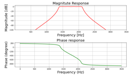
Paso 7: Trazado de la respuesta de fase y magnitud
Python3
# Call mfreqz to plot the magnitude and phase response
mfreqz(z, p, Fs)
Producción:
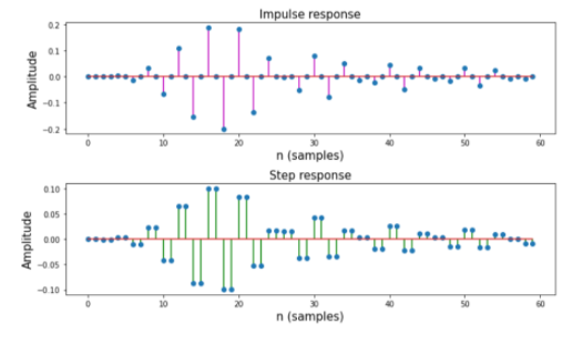
Paso 8: Trazar el impulso y la respuesta al paso
Python3
# Call impz function to plot impulse
# and step response of the filter
impz(z,p)
Producción:
Código completo:
Python3
# import required library
import numpy as np
import scipy.signal as signal
import matplotlib.pyplot as plt


def mfreqz(b, a, Fs):

    # Compute frequency response of the filter
    # using signal.freqz function
    wz, hz = signal.freqz(b, a)

    # Calculate Magnitude from hz in dB
    Mag = 20*np.log10(abs(hz))

    # Calculate phase angle in degree from hz
    Phase = np.unwrap(np.arctan2(np.imag(hz), np.real(hz)))*(180/np.pi)

    # Calculate frequency in Hz from wz
    Freq = wz*Fs/(2*np.pi)

    # Plot filter magnitude and phase responses using subplot.
    fig = plt.figure(figsize=(10, 6))

    # Plot Magnitude response
    sub1 = plt.subplot(2, 1, 1)
    sub1.plot(Freq, Mag, 'r', linewidth=2)
    sub1.axis([1, Fs/2, -100, 5])
    sub1.set_title('Magnitude Response', fontsize=20)
    sub1.set_xlabel('Frequency [Hz]', fontsize=20)
    sub1.set_ylabel('Magnitude [dB]', fontsize=20)
    sub1.grid()

    # Plot phase angle
    sub2 = plt.subplot(2, 1, 2)
    sub2.plot(Freq, Phase, 'g', linewidth=2)
    sub2.set_ylabel('Phase (degree)', fontsize=20)
    sub2.set_xlabel(r'Frequency (Hz)', fontsize=20)
    sub2.set_title(r'Phase response', fontsize=20)
    sub2.grid()

    plt.subplots_adjust(hspace=0.5)
    fig.tight_layout()
    plt.show()

# Define impz(b,a) to calculate impulse response
# and step response of a system
# input: b= an array containing numerator coefficients,
# a= an array containing denominator coefficients
def impz(b, a):

    # Define the impulse sequence of length 60
    impulse = np.repeat(0., 60)
    impulse[0] = 1.
    x = np.arange(0, 60)

    # Compute the impulse response
    response = signal.lfilter(b, a, impulse)

    # Plot filter impulse and step response:
    fig = plt.figure(figsize=(10, 6))
    plt.subplot(211)
    plt.stem(x, response, 'm', use_line_collection=True)
    plt.ylabel('Amplitude', fontsize=15)
    plt.xlabel(r'n (samples)', fontsize=15)
    plt.title(r'Impulse response', fontsize=15)

    plt.subplot(212)
    step = np.cumsum(response)  # Compute step response of the system
    plt.stem(x, step, 'g', use_line_collection=True)
    plt.ylabel('Amplitude', fontsize=15)
    plt.xlabel(r'n (samples)', fontsize=15)
    plt.title(r'Step response', fontsize=15)
    plt.subplots_adjust(hspace=0.5)

    fig.tight_layout()
    plt.show()


# Given specification
Fs = 7000  # Sampling frequency in Hz
fp = np.array([1400, 2100])  # Pass band frequency in Hz
fs = np.array([1050, 2450])  # Stop band frequency in Hz
Ap = 0.4  # Pass band ripple in dB
As = 50  # stop band attenuation in dB


# Compute pass band and stop band edge frequencies
wp = fp/(Fs/2)  # Normalized passband edge frequencies w.r.t. Nyquist rate
ws = fs/(Fs/2)  # Normalized stopband edge frequencies

# Compute order of the  Chebyshev type-1
# filter using signal.cheb1ord
N, wc = signal.cheb1ord(wp, ws, Ap, As)

# Print the order of the filter and cutoff frequencies
print('Order of the filter=', N)
print('Cut-off frequency=', wc)

# Design digital Chebyshev type-1 filter using
# signal.cheby1 function
z, p = signal.cheby1(N, Ap, wc, 'bandpass')


# Print numerator and denomerator coefficients of the filter
print('Numerator Coefficients:', z)
print('Denominator Coefficients:', p)

# Call mfreqz to plot the magnitude and phase response
mfreqz(z, p, Fs)

# Call impz function to plot impulse and
# step response of the filter
impz(z, p)
Producción:
Publicación traducida automáticamente
Artículo escrito por sagnikmukherjee2 y traducido por Barcelona Geeks. The original can be accessed here. Licence: CCBY-SA