Filtro digital de paso bajo Butterworth en Python

En este artículo, vamos a discutir cómo diseñar un filtro Butterworth de paso bajo digital usando Python. El filtro Butterworth es un tipo de filtro de procesamiento de señal diseñado para tener una respuesta de frecuencia lo más plana posible en la banda de paso. Tomemos las siguientes especificaciones para diseñar el filtro y observar la respuesta de magnitud, fase e impulso del filtro digital Butterworth.

Las especificaciones son las siguientes: 

• Tasa de muestreo de 40 kHz
• Frecuencia de borde de banda de paso de 4 kHz
• Frecuencia de borde de banda de parada de 8kHz
• Ondulación de banda de paso de 0,5 dB
• Atenuación mínima de la banda de parada de 40 dB

Graficaremos la respuesta de magnitud, fase e impulso del filtro.

Enfoque paso a paso:

Paso 1: Importación de todas las bibliotecas necesarias.

# import required modules
import numpy as np
import matplotlib.pyplot as plt
from scipy import signal
import math

Paso 2: Definir variables con las especificaciones dadas del filtro.

# Specifications of Filter
  
 # sampling frequency
f_sample = 40000 
  
# pass band frequency
f_pass = 4000  
  
# stop band frequency
f_stop = 8000  
  
# pass band ripple
fs = 0.5
  
# pass band freq in radian
wp = f_pass/(f_sample/2)  
  
# stop band freq in radian
ws = f_stop/(f_sample/2) 
  
# Sampling Time
Td = 1  
  
 # pass band ripple
g_pass = 0.5 
  
# stop band attenuation
g_stop = 40  

Paso 3: Construcción del filtro usando la función signal.buttord .

# Conversion to prewrapped analog frequency
omega_p = (2/Td)*np.tan(wp/2)
omega_s = (2/Td)*np.tan(ws/2)
  
  
# Design of Filter using signal.buttord function
N, Wn = signal.buttord(omega_p, omega_s, g_pass, g_stop, analog=True)
  
  
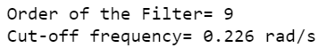
# Printing the values of order & cut-off frequency!
print("Order of the Filter=", N)  # N is the order
# Wn is the cut-off freq of the filter
print("Cut-off frequency= {:.3f} rad/s ".format(Wn))
  
  
# Conversion in Z-domain
  
# b is the numerator of the filter & a is the denominator
b, a = signal.butter(N, Wn, 'low', True)
z, p = signal.bilinear(b, a, fs)
# w is the freq in z-domain & h is the magnitude in z-domain
w, h = signal.freqz(z, p, 512)

Producción:

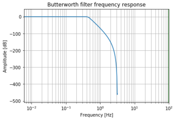
Paso 4: Trazado de la Respuesta de Magnitud.

# Magnitude Response
plt.semilogx(w, 20*np.log10(abs(h)))
plt.xscale('log')
plt.title('Butterworth filter frequency response')
plt.xlabel('Frequency [Hz]')
plt.ylabel('Amplitude [dB]')
plt.margins(0, 0.1)
plt.grid(which='both', axis='both')
plt.axvline(100, color='green')
plt.show()

Producción:

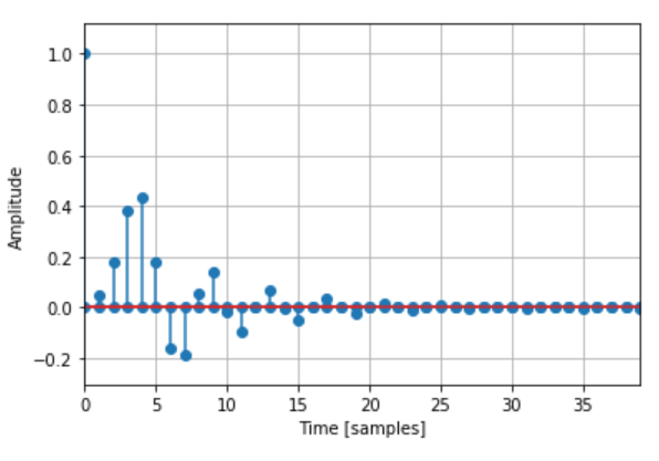
Paso 5: Representación gráfica de la respuesta al impulso.

# Impulse Response
imp = signal.unit_impulse(40)
c, d = signal.butter(N, 0.5)
response = signal.lfilter(c, d, imp)
  
plt.stem(np.arange(0, 40), imp, use_line_collection=True)
plt.stem(np.arange(0, 40), response, use_line_collection=True)
plt.margins(0, 0.1)
  
plt.xlabel('Time [samples]')
plt.ylabel('Amplitude')
plt.grid(True)
plt.show()

Producción:

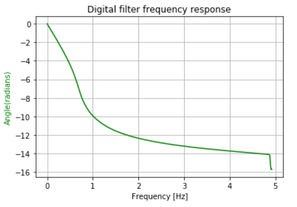
Paso 6: Trazado de la respuesta de fase.

# Phase Response
fig, ax1 = plt.subplots()
  
ax1.set_title('Digital filter frequency response')
ax1.set_ylabel('Angle(radians)', color='g')
ax1.set_xlabel('Frequency [Hz]')
  
angles = np.unwrap(np.angle(h))
  
ax1.plot(w/2*np.pi, angles, 'g')
ax1.grid()
ax1.axis('tight')
plt.show()

Producción:

A continuación se muestra el programa completo basado en el enfoque anterior:

# import required modules
import numpy as np
import matplotlib.pyplot as plt
from scipy import signal
import math
  
  
# Specifications of Filter
  
 # sampling frequency
f_sample = 40000 
  
# pass band frequency
f_pass = 4000  
  
# stop band frequency
f_stop = 8000  
  
# pass band ripple
fs = 0.5
  
# pass band freq in radian
wp = f_pass/(f_sample/2)  
  
# stop band freq in radian
ws = f_stop/(f_sample/2) 
  
# Sampling Time
Td = 1  
  
 # pass band ripple
g_pass = 0.5 
  
# stop band attenuation
g_stop = 40  
  
  
# Conversion to prewrapped analog frequency
omega_p = (2/Td)*np.tan(wp/2)
omega_s = (2/Td)*np.tan(ws/2)
  
  
# Design of Filter using signal.buttord function
N, Wn = signal.buttord(omega_p, omega_s, g_pass, g_stop, analog=True)
  
  
# Printing the values of order & cut-off frequency!
print("Order of the Filter=", N)  # N is the order
# Wn is the cut-off freq of the filter
print("Cut-off frequency= {:.3f} rad/s ".format(Wn))
  
  
# Conversion in Z-domain
  
# b is the numerator of the filter & a is the denominator
b, a = signal.butter(N, Wn, 'low', True)
z, p = signal.bilinear(b, a, fs)
# w is the freq in z-domain & h is the magnitude in z-domain
w, h = signal.freqz(z, p, 512)
  
  
# Magnitude Response
plt.semilogx(w, 20*np.log10(abs(h)))
plt.xscale('log')
plt.title('Butterworth filter frequency response')
plt.xlabel('Frequency [Hz]')
plt.ylabel('Amplitude [dB]')
plt.margins(0, 0.1)
plt.grid(which='both', axis='both')
plt.axvline(100, color='green')
plt.show()
  
  
# Impulse Response
imp = signal.unit_impulse(40)
c, d = signal.butter(N, 0.5)
response = signal.lfilter(c, d, imp)
plt.stem(np.arange(0, 40), imp, use_line_collection=True)
plt.stem(np.arange(0, 40), response, use_line_collection=True)
plt.margins(0, 0.1)
plt.xlabel('Time [samples]')
plt.ylabel('Amplitude')
plt.grid(True)
plt.show()
  
  
# Phase Response
fig, ax1 = plt.subplots()
ax1.set_title('Digital filter frequency response')
ax1.set_ylabel('Angle(radians)', color='g')
ax1.set_xlabel('Frequency [Hz]')
angles = np.unwrap(np.angle(h))
ax1.plot(w/2*np.pi, angles, 'g')
ax1.grid()
ax1.axis('tight')
plt.show()

Producción: