Matrix es un arreglo rectangular de números en filas y columnas. En una array, como sabemos, las filas son las que se ejecutan horizontalmente y las columnas son las que se ejecutan verticalmente. En R, las arrays son estructuras de datos bidimensionales y homogéneas. Estos son algunos ejemplos de arrays.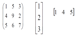
Las operaciones algebraicas básicas son cualquiera de las operaciones aritméticas tradicionales, que son la suma, la resta, la multiplicación, la división, la elevación a una potencia entera y la extracción de raíces. Estas operaciones pueden realizarse con números, en cuyo caso a menudo se denominan operaciones aritméticas. Podemos realizar muchas más operaciones algebraicas sobre una array en R. Operaciones algebraicas que se pueden realizar sobre una array en R:
- Operaciones en una sola array
- operaciones unarias
- Operaciones binarias
- Operaciones algebraicas lineales
- Rango, determinante, transpuesta, inversa, traza de una array
- Nulidad de una array
- Valores propios y vectores propios de arrays
- Resolver una ecuación matricial lineal
Operaciones en una sola array
Podemos usar operadores aritméticos sobrecargados para realizar operaciones por elementos en una array para crear una nueva array. En el caso de los operadores +=, -=, *=, se modifica la array existente.
Python3
# R program to demonstrate
# basic operations on a single matrix

# Create a 3x3 matrix
a = matrix(
  c(1, 2, 3, 4, 5, 6, 7, 8, 9),
  nrow = 3,
  ncol = 3,
  byrow = TRUE
)
cat("The 3x3 matrix:\n")
print(a)

# add 1 to every element
cat("Adding 1 to every element:\n")
print(a + 1)

# subtract 3 from each element
cat("Subtracting 3 from each element:\n")
print(a-3)

# multiply each element by 10
cat("Multiplying each element by 10:\n")
print(a * 10)

# square each element
cat("Squaring each element:\n")
print(a ^ 2)

# modify existing matrix
cat("Doubled each element of original matrix:\n")
print(a * 2)
Producción:
The 3x3 matrix:
     [, 1] [, 2] [, 3]
[1, ]    1    2    3
[2, ]    4    5    6
[3, ]    7    8    9
Adding 1 to every element:
     [, 1] [, 2] [, 3]
[1, ]    2    3    4
[2, ]    5    6    7
[3, ]    8    9   10
Subtracting 3 from each element:
     [, 1] [, 2] [, 3]
[1, ]   -2   -1    0
[2, ]    1    2    3
[3, ]    4    5    6
Multiplying each element by 10:
     [, 1] [, 2] [, 3]
[1, ]   10   20   30
[2, ]   40   50   60
[3, ]   70   80   90
Squaring each element:
     [, 1] [, 2] [, 3]
[1, ]    1    4    9
[2, ]   16   25   36
[3, ]   49   64   81
Doubled each element of original matrix:
     [, 1] [, 2] [, 3]
[1, ]    2    4    6
[2, ]    8   10   12
[3, ]   14   16   18
operaciones unarias
Se pueden realizar muchas operaciones unarias en una array en R. Esto incluye sum, min, max, etc.
Python3
# R program to demonstrate
# unary operations on a matrix

# Create a 3x3 matrix
a = matrix(
  c(1, 2, 3, 4, 5, 6, 7, 8, 9),
  nrow = 3,
  ncol = 3,
  byrow = TRUE
)
cat("The 3x3 matrix:\n")
print(a)

# maximum element in the matrix
cat("Largest element is:\n")
print(max(a))

# minimum element in the matrix
cat("Smallest element is:\n")
print(min(a))

# sum of element in the matrix
cat("Sum of elements is:\n")
print(sum(a))
Producción:
The 3x3 matrix:
     [, 1] [, 2] [, 3]
[1, ]    1    2    3
[2, ]    4    5    6
[3, ]    7    8    9
Largest element is:
[1] 9
Smallest element is:
[1] 1
Sum of elements is:
[1] 45
Operaciones binarias
Estas operaciones se aplican en una array por elementos y se crea una nueva array. Puede utilizar todos los operadores aritméticos básicos como +, -, *, /, etc. En el caso de los operadores +=, -=, =, se modifica la array existente.
Python3
# R program to demonstrate
# binary operations on a matrix

# Create a 3x3 matrix
a = matrix(
  c(1, 2, 3, 4, 5, 6, 7, 8, 9),
  nrow = 3,
  ncol = 3,
  byrow = TRUE
)
cat("The 3x3 matrix:\n")
print(a)

# Create another 3x3 matrix
b = matrix(
  c(1, 2, 5, 4, 6, 2, 9, 4, 3),
  nrow = 3,
  ncol = 3,
  byrow = TRUE
)
cat("The another 3x3 matrix:\n")
print(b)

cat("Matrix addition:\n")
print(a + b)

cat("Matrix subtraction:\n")
print(a-b)

cat("Matrix element wise multiplication:\n")
print(a * b)

cat("Regular Matrix multiplication:\n")
print(a %*% b)

cat("Matrix elementwise division:\n")
print(a / b)
Producción:
The 3x3 matrix:
     [, 1] [, 2] [, 3]
[1, ]    1    2    3
[2, ]    4    5    6
[3, ]    7    8    9
The another 3x3 matrix:
     [, 1] [, 2] [, 3]
[1, ]    1    2    5
[2, ]    4    6    2
[3, ]    9    4    3
Matrix addition:
     [, 1] [, 2] [, 3]
[1, ]    2    4    8
[2, ]    8   11    8
[3, ]   16   12   12
Matrix subtraction:
     [, 1] [, 2] [, 3]
[1, ]    0    0   -2
[2, ]    0   -1    4
[3, ]   -2    4    6
Matrix element wise multiplication:
     [, 1] [, 2] [, 3]
[1, ]    1    4   15
[2, ]   16   30   12
[3, ]   63   32   27
Regular Matrix multiplication:
     [, 1] [, 2] [, 3]
[1, ]   36   26   18
[2, ]   78   62   48
[3, ]  120   98   78
Matrix elementwise division:
          [, 1]      [, 2] [, 3]
[1, ] 1.0000000 1.0000000  0.6
[2, ] 1.0000000 0.8333333  3.0
[3, ] 0.7777778 2.0000000  3.0
Operaciones algebraicas lineales
Se pueden realizar muchas operaciones algebraicas lineales en una array dada en R. Algunas de ellas son las siguientes:
- Rango, determinante, transpuesta, inversa, traza de una array:
Python3
# R program to demonstrate
# Linear algebraic operations on a matrix

# Importing required library
library(pracma) # For rank of matrix
library(psych)  # For trace of matrix

# Create a 3x3 matrix
A = matrix(
  c(6, 1, 1, 4, -2, 5, 2, 8, 7),
  nrow = 3,
  ncol = 3,
  byrow = TRUE
)
cat("The 3x3 matrix:\n")
print(A)

# Rank of a matrix
cat("Rank of A:\n")
print(Rank(A))

# Trace of matrix A
cat("Trace of A:\n")
print(tr(A))

# Determinant of a matrix
cat("Determinant of A:\n")
print(det(A))

# Transpose of a matrix
cat("Transpose of A:\n")
print(t(A))

# Inverse of matrix A
cat("Inverse of A:\n")
print(inv(A))
- Producción:
The 3x3 matrix:
     [, 1] [, 2] [, 3]
[1, ]    6    1    1
[2, ]    4   -2    5
[3, ]    2    8    7
Rank of A:
[1] 3
Trace of A:
[1] 11
Determinant of A:
[1] -306
Transpose of A:
     [, 1] [, 2] [, 3]
[1, ]    6    4    2
[2, ]    1   -2    8
[3, ]    1    5    7
Inverse of A:
            [, 1]         [, 2]        [, 3]
[1, ]  0.17647059 -0.003267974 -0.02287582
[2, ]  0.05882353 -0.130718954  0.08496732
[3, ] -0.11764706  0.150326797  0.05228758
- Nulidad de una array:
Python3
# R program to demonstrate
# nullity of a matrix

# Importing required library
library(pracma)

# Create a 3x3 matrix
a = matrix(
  c(1, 2, 3, 4, 5, 6, 7, 8, 9),
  nrow = 3,
  ncol = 3,
  byrow = TRUE
)
cat("The 3x3 matrix:\n")
print(a)

# No of column
col = ncol(a)

# Rank of matrix
rank = Rank(a)

# Calculating nullity
nullity = col - rank

cat("Nullity of matrix is:\n")
print(nullity)
- Producción:
The 3x3 matrix:
     [, 1] [, 2] [, 3]
[1, ]    1    2    3
[2, ]    4    5    6
[3, ]    7    8    9
Nullity of matrix is:
[1] 1
- Valores propios y vectores propios de arrays:
Python3
# R program to illustrate
# Eigenvalues and eigenvectors of metrics

# Create a 3x3 matrix
A = matrix(
  c(1, 2, 3, 4, 5, 6, 7, 8, 9),
  nrow = 3,
  ncol = 3,
  byrow = TRUE
)
cat("The 3x3 matrix:\n")
print(A)

# Calculating Eigenvalues and eigenvectors
print(eigen(A))
- Producción:
The 3x3 matrix:
     [, 1] [, 2] [, 3]
[1, ]    1    2    3
[2, ]    4    5    6
[3, ]    7    8    9
eigen() decomposition
$values
[1]  1.611684e+01 -1.116844e+00 -1.303678e-15

$vectors
           [, 1]        [, 2]       [, 3]
[1, ] -0.2319707 -0.78583024  0.4082483
[2, ] -0.5253221 -0.08675134 -0.8164966
[3, ] -0.8186735  0.61232756  0.4082483
- Resolver una ecuación matricial lineal:
Python3
# R program to illustrate
# Solve a linear matrix equation of metrics

# Importing library for applying pseudoinverse
library(MASS)

# Create a 2x2 matrix
A = matrix(
  c(1, 2, 3, 4),
  nrow = 2,
  ncol = 2,
)
cat("A = :\n")
print(A)

# Create another 2x1 matrix
b = matrix(
  c(7, 10),
  nrow = 2,
  ncol = 1,
)
cat("b = :\n")
print(b)

cat("Solution of linear equations:\n")
print(solve(A)%*% b)

cat("Solution of linear equations using pseudoinverse:\n")
print(ginv(A)%*% b)
- Producción:
A = :
     [, 1] [, 2]
[1, ]    1    3
[2, ]    2    4
b = :
     [, 1]
[1, ]    7
[2, ]   10
Solution of linear equations:
     [, 1]
[1, ]    1
[2, ]    2
Solution of linear equations using pseudoinverse:
     [, 1]
[1, ]    1
[2, ]    2
Publicación traducida automáticamente
Artículo escrito por AmiyaRanjanRout y traducido por Barcelona Geeks. The original can be accessed here. Licence: CCBY-SA