ML | OPTICS Clustering Implementación usando Sklearn

import numpy as np
import pandas as pd
import matplotlib.pyplot as plt
from matplotlib import gridspec
from sklearn.cluster import OPTICS, cluster_optics_dbscan
from sklearn.preprocessing import normalize, StandardScaler

# Changing the working location to the location of the data
cd C:\Users\Dev\Desktop\Kaggle\Customer Segmentation
  
X = pd.read_csv('Mall_Customers.csv')
  
# Dropping irrelevant columns
drop_features = ['CustomerID', 'Gender']
X = X.drop(drop_features, axis = 1)
  
# Handling the missing values if any
X.fillna(method ='ffill', inplace = True)
  
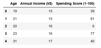
X.head()

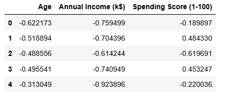
# Scaling the data to bring all the attributes to a comparable level
scaler = StandardScaler()
X_scaled = scaler.fit_transform(X)
  
# Normalizing the data so that the data
# approximately follows a Gaussian distribution
X_normalized = normalize(X_scaled)
  
# Converting the numpy array into a pandas DataFrame
X_normalized = pd.DataFrame(X_normalized)
  
# Renaming the columns
X_normalized.columns = X.columns
  
X_normalized.head()

# Building the OPTICS Clustering model
optics_model = OPTICS(min_samples = 10, xi = 0.05, min_cluster_size = 0.05)
  
# Training the model
optics_model.fit(X_normalized)

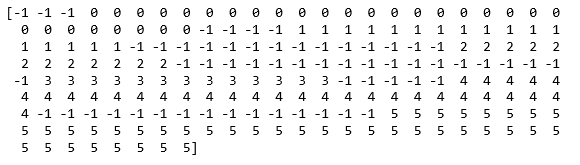
# Producing the labels according to the DBSCAN technique with eps = 0.5
labels1 = cluster_optics_dbscan(reachability = optics_model.reachability_,
                                   core_distances = optics_model.core_distances_,
                                   ordering = optics_model.ordering_, eps = 0.5)
  
# Producing the labels according to the DBSCAN technique with eps = 2.0
labels2 = cluster_optics_dbscan(reachability = optics_model.reachability_,
                                   core_distances = optics_model.core_distances_,
                                   ordering = optics_model.ordering_, eps = 2)
  
# Creating a numpy array with numbers at equal spaces till
# the specified range
space = np.arange(len(X_normalized))
  
# Storing the reachability distance of each point
reachability = optics_model.reachability_[optics_model.ordering_]
  
# Storing the cluster labels of each point
labels = optics_model.labels_[optics_model.ordering_]
  
print(labels)

# Defining the framework of the visualization
plt.figure(figsize =(10, 7))
G = gridspec.GridSpec(2, 3)
ax1 = plt.subplot(G[0, :])
ax2 = plt.subplot(G[1, 0])
ax3 = plt.subplot(G[1, 1])
ax4 = plt.subplot(G[1, 2])
  
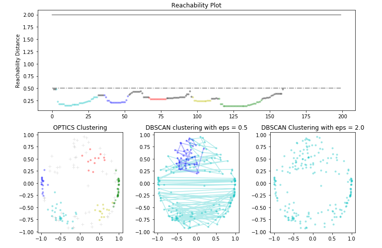
# Plotting the Reachability-Distance Plot
colors = ['c.', 'b.', 'r.', 'y.', 'g.']
for Class, colour in zip(range(0, 5), colors):
    Xk = space[labels == Class]
    Rk = reachability[labels == Class]
    ax1.plot(Xk, Rk, colour, alpha = 0.3)
ax1.plot(space[labels == -1], reachability[labels == -1], 'k.', alpha = 0.3)
ax1.plot(space, np.full_like(space, 2., dtype = float), 'k-', alpha = 0.5)
ax1.plot(space, np.full_like(space, 0.5, dtype = float), 'k-.', alpha = 0.5)
ax1.set_ylabel('Reachability Distance')
ax1.set_title('Reachability Plot')
  
# Plotting the OPTICS Clustering
colors = ['c.', 'b.', 'r.', 'y.', 'g.']
for Class, colour in zip(range(0, 5), colors):
    Xk = X_normalized[optics_model.labels_ == Class]
    ax2.plot(Xk.iloc[:, 0], Xk.iloc[:, 1], colour, alpha = 0.3)
      
ax2.plot(X_normalized.iloc[optics_model.labels_ == -1, 0],
        X_normalized.iloc[optics_model.labels_ == -1, 1],
       'k+', alpha = 0.1)
ax2.set_title('OPTICS Clustering')
  
# Plotting the DBSCAN Clustering with eps = 0.5
colors = ['c', 'b', 'r', 'y', 'g', 'greenyellow']
for Class, colour in zip(range(0, 6), colors):
    Xk = X_normalized[labels1 == Class]
    ax3.plot(Xk.iloc[:, 0], Xk.iloc[:, 1], colour, alpha = 0.3, marker ='.')
        
ax3.plot(X_normalized.iloc[labels1 == -1, 0],
        X_normalized.iloc[labels1 == -1, 1],
       'k+', alpha = 0.1)
ax3.set_title('DBSCAN clustering with eps = 0.5')
  
# Plotting the DBSCAN Clustering with eps = 2.0
colors = ['c.', 'y.', 'm.', 'g.']
for Class, colour in zip(range(0, 4), colors):
    Xk = X_normalized.iloc[labels2 == Class]
    ax4.plot(Xk.iloc[:, 0], Xk.iloc[:, 1], colour, alpha = 0.3)
          
ax4.plot(X_normalized.iloc[labels2 == -1, 0],
        X_normalized.iloc[labels2 == -1, 1],
       'k+', alpha = 0.1)
ax4.set_title('DBSCAN Clustering with eps = 2.0')
  
  
plt.tight_layout()
plt.show()