Prerrequisitos: comprensión de la regresión logística y TensorFlow .
Breve resumen de la regresión
logística: la regresión logística es un algoritmo de clasificación comúnmente utilizado en el aprendizaje automático. Permite categorizar datos en clases discretas aprendiendo la relación de un conjunto dado de datos etiquetados. Aprende una relación lineal del conjunto de datos dado y luego introduce una no linealidad en forma de función sigmoidea.
En caso de regresión Logística, la hipótesis es el Sigmoide de una línea recta, es decir,  donde
donde 
el vector wrepresenta los Pesos y el escalar brepresenta el Sesgo del modelo.
Visualicemos la función sigmoidea:
import numpy as np
import matplotlib.pyplot as plt

def sigmoid(z):
    return 1 / (1 + np.exp( - z))

plt.plot(np.arange(-5, 5, 0.1), sigmoid(np.arange(-5, 5, 0.1)))
plt.title('Visualization of the Sigmoid Function')

plt.show()
Salida: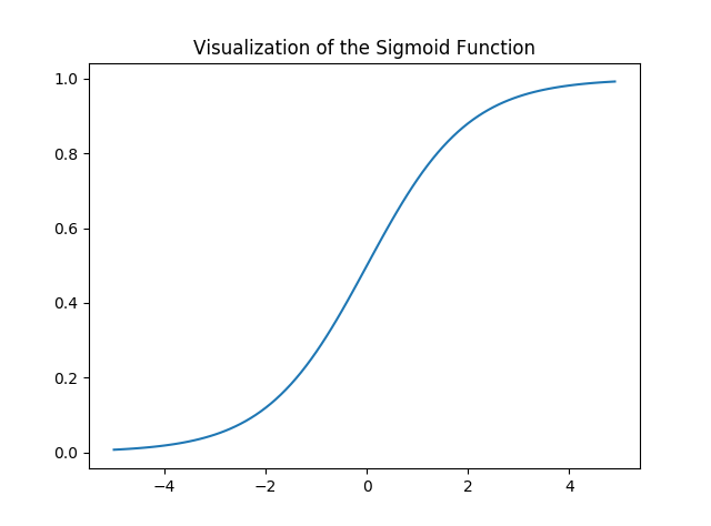
tenga en cuenta que el rango de la función Sigmoid es (0, 1), lo que significa que los valores resultantes están entre 0 y 1. Esta propiedad de la función Sigmoid la convierte en una muy buena opción de función de activación para la clasificación binaria. También for z = 0, Sigmoid(z) = 0.5cuál es el punto medio del rango de la función sigmoidea.
Al igual que la regresión lineal, necesitamos encontrar los valores óptimos de w y b para los cuales la función de costo J es mínima. En este caso, usaremos la función de costo Sigmoid Cross Entropy que está dada por 
Esta función de costo luego se optimizará usando Gradient Descent.
Implementación:
Comenzaremos importando las bibliotecas necesarias. Usaremos Numpy junto con Tensorflow para los cálculos, Pandas para el análisis básico de datos y Matplotlib para el trazado. También utilizaremos el módulo de preprocesamiento de Scikit-LearnOne Hot Encoding de los datos.
# importing modules
import numpy as np
import pandas as pd
import tensorflow as tf
import matplotlib.pyplot as plt
from sklearn.preprocessing import OneHotEncoder
A continuación, importaremos el conjunto de datos . Usaremos un subconjunto del famoso conjunto de datos Iris .
data = pd.read_csv('dataset.csv', header = None)
print("Data Shape:", data.shape)

print(data.head())
Producción:
Data Shape: (100, 4)
   0    1    2  3
0  0  5.1  3.5  1
1  1  4.9  3.0  1
2  2  4.7  3.2  1
3  3  4.6  3.1  1
4  4  5.0  3.6  1
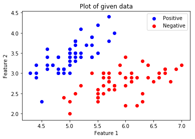
Ahora obtengamos la array de características y las etiquetas correspondientes y visualicemos.
# Feature Matrix
x_orig = data.iloc[:, 1:-1].values

# Data labels
y_orig = data.iloc[:, -1:].values

print("Shape of Feature Matrix:", x_orig.shape)
print("Shape Label Vector:", y_orig.shape)
Producción:
Shape of Feature Matrix: (100, 2)
Shape Label Vector: (100, 1)
Visualiza los datos dados.
# Positive Data Points
x_pos = np.array([x_orig[i] for i in range(len(x_orig))
                                    if y_orig[i] == 1])

# Negative Data Points
x_neg = np.array([x_orig[i] for i in range(len(x_orig))
                                    if y_orig[i] == 0])

# Plotting the Positive Data Points
plt.scatter(x_pos[:, 0], x_pos[:, 1], color = 'blue', label = 'Positive')

# Plotting the Negative Data Points
plt.scatter(x_neg[:, 0], x_neg[:, 1], color = 'red', label = 'Negative')

plt.xlabel('Feature 1')
plt.ylabel('Feature 2')
plt.title('Plot of given data')
plt.legend()

plt.show()
 .
.
Ahora seremos One Hot Encoding los datos para que funcionen con el algoritmo. Una codificación en caliente transforma características categóricas a un formato que funciona mejor con algoritmos de clasificación y regresión. También estableceremos la tasa de aprendizaje y el número de épocas.
# Creating the One Hot Encoder
oneHot = OneHotEncoder()

# Encoding x_orig
oneHot.fit(x_orig)
x = oneHot.transform(x_orig).toarray()

# Encoding y_orig
oneHot.fit(y_orig)
y = oneHot.transform(y_orig).toarray()

alpha, epochs = 0.0035, 500
m, n = x.shape
print('m =', m)
print('n =', n)
print('Learning Rate =', alpha)
print('Number of Epochs =', epochs)
Producción:
m = 100
n = 7
Learning Rate = 0.0035
Number of Epochs = 500
Ahora comenzaremos a crear el modelo definiendo los marcadores de posición Xy Y, para que podamos alimentar nuestros ejemplos de entrenamiento xy yel optimizador durante el proceso de entrenamiento. También crearemos las Variables entrenables Wy bque pueden ser optimizadas por el Optimizador de Descenso de Gradiente.
# There are n columns in the feature matrix
# after One Hot Encoding.
X = tf.placeholder(tf.float32, [None, n])

# Since this is a binary classification problem,
# Y can take only 2 values.
Y = tf.placeholder(tf.float32, [None, 2])

# Trainable Variable Weights
W = tf.Variable(tf.zeros([n, 2]))

# Trainable Variable Bias
b = tf.Variable(tf.zeros([2]))
Ahora declare la hipótesis, la función de costo, el optimizador y el inicializador de variables globales.
# Hypothesis
Y_hat = tf.nn.sigmoid(tf.add(tf.matmul(X, W), b))

# Sigmoid Cross Entropy Cost Function
cost = tf.nn.sigmoid_cross_entropy_with_logits(
                    logits = Y_hat, labels = Y)

# Gradient Descent Optimizer
optimizer = tf.train.GradientDescentOptimizer(
         learning_rate = alpha).minimize(cost)

# Global Variables Initializer
init = tf.global_variables_initializer()
Comienza el proceso de entrenamiento dentro de una sesión de Tensorflow.
# Starting the Tensorflow Session
with tf.Session() as sess:

    # Initializing the Variables
    sess.run(init)

    # Lists for storing the changing Cost and Accuracy in every Epoch
    cost_history, accuracy_history = [], []

    # Iterating through all the epochs
    for epoch in range(epochs):
        cost_per_epoch = 0

        # Running the Optimizer
        sess.run(optimizer, feed_dict = {X : x, Y : y})

        # Calculating cost on current Epoch
        c = sess.run(cost, feed_dict = {X : x, Y : y})

        # Calculating accuracy on current Epoch
        correct_prediction = tf.equal(tf.argmax(Y_hat, 1),
                                          tf.argmax(Y, 1))
        accuracy = tf.reduce_mean(tf.cast(correct_prediction,
                                                 tf.float32))

        # Storing Cost and Accuracy to the history
        cost_history.append(sum(sum(c)))
        accuracy_history.append(accuracy.eval({X : x, Y : y}) * 100)

        # Displaying result on current Epoch
        if epoch % 100 == 0 and epoch != 0:
            print("Epoch " + str(epoch) + " Cost: "
                            + str(cost_history[-1]))

    Weight = sess.run(W) # Optimized Weight
    Bias = sess.run(b)   # Optimized Bias

    # Final Accuracy
    correct_prediction = tf.equal(tf.argmax(Y_hat, 1),
                                      tf.argmax(Y, 1))
    accuracy = tf.reduce_mean(tf.cast(correct_prediction,
                                             tf.float32))
    print("\nAccuracy:", accuracy_history[-1], "%")
Producción:
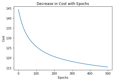
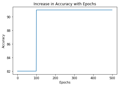
Epoch 100 Cost: 125.700202942
Epoch 200 Cost: 120.647117615
Epoch 300 Cost: 118.151592255
Epoch 400 Cost: 116.549999237

Accuracy: 91.0000026226 %
Grafiquemos el cambio de costo sobre las épocas.
plt.plot(list(range(epochs)), cost_history)
plt.xlabel('Epochs')
plt.ylabel('Cost')
plt.title('Decrease in Cost with Epochs')

plt.show()
Trazar el cambio de precisión sobre las épocas.
plt.plot(list(range(epochs)), accuracy_history)
plt.xlabel('Epochs')
plt.ylabel('Accuracy')
plt.title('Increase in Accuracy with Epochs')

plt.show()
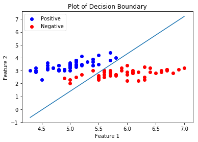
Ahora estaremos trazando el límite de decisión para nuestro clasificador entrenado. Un límite de decisión es una hipersuperficie que divide el espacio vectorial subyacente en dos conjuntos, uno para cada clase.
# Calculating the Decision Boundary
decision_boundary_x = np.array([np.min(x_orig[:, 0]),
                               np.max(x_orig[:, 0])])

decision_boundary_y = (- 1.0 / Weight[0]) *
      (decision_boundary_x * Weight + Bias)

decision_boundary_y = [sum(decision_boundary_y[:, 0]),
                       sum(decision_boundary_y[:, 1])]

# Positive Data Points
x_pos = np.array([x_orig[i] for i in range(len(x_orig))
                                    if y_orig[i] == 1])

# Negative Data Points
x_neg = np.array([x_orig[i] for i in range(len(x_orig))
                                    if y_orig[i] == 0])

# Plotting the Positive Data Points
plt.scatter(x_pos[:, 0], x_pos[:, 1],
  color = 'blue', label = 'Positive')

# Plotting the Negative Data Points
plt.scatter(x_neg[:, 0], x_neg[:, 1],
   color = 'red', label = 'Negative')

# Plotting the Decision Boundary
plt.plot(decision_boundary_x, decision_boundary_y)
plt.xlabel('Feature 1')
plt.ylabel('Feature 2')
plt.title('Plot of Decision Boundary')
plt.legend()

plt.show()
Publicación traducida automáticamente
Artículo escrito por geekyRakshit y traducido por Barcelona Geeks. The original can be accessed here. Licence: CCBY-SA