Python Bokeh es una biblioteca de visualización de datos que proporciona gráficos y diagramas interactivos. Bokeh representa sus tramas utilizando HTML y JavaScript que utilizan navegadores web modernos para presentar una construcción elegante y concisa de gráficos novedosos con interactividad de alto nivel.
Características de Bokeh:
- Flexibilidad: Bokeh se puede utilizar para requisitos de trazado comunes y para casos de uso personalizados y complejos.
- Productividad: Su interacción con otras herramientas populares de Pydata (como Pandas y Jupyter notebook) es muy fácil.
- Interactividad: Crea tramas interactivas que cambian con la interacción del usuario.
- Potente: la generación de visualizaciones para casos de uso especializados se puede realizar agregando JavaScript.
- Compartible: los datos visuales se pueden compartir. También se pueden representar en cuadernos Jupyter.
- Código abierto: Bokeh es un proyecto de código abierto.

Este tutorial tiene como objetivo proporcionar información sobre Bokeh utilizando conceptos y ejemplos bien explicados con la ayuda de un gran conjunto de datos. Así que profundicemos en el Bokeh y aprendamos todo, desde lo básico hasta lo avanzado.
Tabla de contenidos
- Instalación
- Interfaces de Bokeh: conceptos básicos de Bokeh
- Empezando
- Anotaciones y Leyendas
- Trazado de diferentes tipos de gráficos
- Creando diferentes formas
- Trazado de múltiples parcelas
- Visualización interactiva de datos
- Crear diferentes tipos de glifos
- Visualización de diferentes tipos de datos
- Más temas sobre Bokeh
Instalación
Bokeh es compatible con CPython 3.6 y versiones anteriores con distribución estándar y distribución anaconda. El paquete Bokeh tiene las siguientes dependencias.
1. Dependencias requeridas
- PyYAML>=3.10
- python-dateutil>=2.1
- Jinja2>=2.7
- numpy>=1.11.3
- Pillow>=4.0
- embalaje>=16.8
- tornado>=5
- escribiendo_extensiones >=3.7.4
2. Dependencias opcionales
- Jupyter
- NodeJS
- RedX
- pandas
- psutil
- Selenium, GeckoDriver, Firefox
- Esfinge
Bokeh se puede instalar usando el administrador de paquetes conda y pip. Para instalarlo usando conda, escriba el siguiente comando en la terminal.
conda install bokeh
Esto instalará todas las dependencias. Si todas las dependencias están instaladas, puede instalar el bokeh desde PyPI usando pip. Escriba el siguiente comando en la terminal.
pip install bokeh
Consulte el siguiente artículo para obtener información detallada sobre la instalación de Bokeh.
Interfaces de Bokeh: conceptos básicos de Bokeh
Bokeh es fácil de usar, ya que proporciona una interfaz simple para los científicos de datos que no quieren distraerse con su implementación y también proporciona una interfaz detallada para desarrolladores e ingenieros de software que deseen tener más control sobre Bokeh para crear funciones más sofisticadas. Para hacer esto, Bokeh sigue el enfoque en capas.
Bokeh.modelos
Esta clase es la biblioteca de Python para Bokeh que contiene clases modelo que manejan los datos JSON creados por la biblioteca de JavaScript de Bokeh (BokehJS). La mayoría de los modelos son muy básicos y consisten en muy pocos atributos o ningún método.
bokeh.trazado
Esta es la interfaz de nivel medio que proporciona funciones similares a Matplotlib o MATLAB para el trazado. Se ocupa de los datos que se van a trazar y de la creación de ejes, cuadrículas y herramientas válidos. La clase principal de esta interfaz es la clase Figure .
Empezando
Después de la instalación y de aprender los conceptos básicos de Bokeh, creemos una trama simple.
Ejemplo:
Python3
# importing the modules
from bokeh.plotting import figure, output_file, show

# instantiating the figure object
graph = figure(title = "Bokeh Line Graph")

# the points to be plotted
x = [1, 2, 3, 4, 5]
y = [5, 4, 3, 2, 1]

# plotting the line graph
graph.line(x, y)

# displaying the model
show(graph)
Producción:
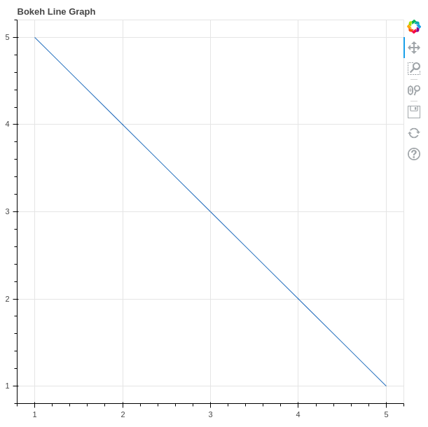
En el ejemplo anterior, hemos creado un gráfico simple con el título como gráfico de líneas Bokeh. Si está utilizando Jupyter, la salida se creará en una nueva pestaña en el navegador.
Anotaciones y Leyendas
Las anotaciones son la información complementaria, como títulos, leyendas, flechas , etc., que se pueden agregar a los gráficos. En el ejemplo anterior, ya hemos visto cómo agregar los títulos al gráfico. En esta sección, veremos acerca de las leyendas.
Agregar leyendas a sus figuras puede ayudar a describirlas y definirlas correctamente. Por lo tanto, dando más claridad. Las leyendas en Bokeh son fáciles de implementar. Pueden ser básicos, agrupados automáticamente, mencionados manualmente, indexados explícitamente y también interactivos.
Ejemplo:
Python3
# importing the modules
from bokeh.plotting import figure, output_file, show

# instantiating the figure object
graph = figure(title="Bokeh Line Graph")

# the points to be plotted
x = [1, 2, 3, 4, 5]
y = [5, 4, 3, 2, 1]

# plotting the 1st line graph
graph.line(x, x, legend_label="Line 1")

# plotting the 2nd line graph with a
# different color
graph.line(y, x, legend_label="Line 2",
           line_color="green")

# displaying the model
show(graph)
Producción:
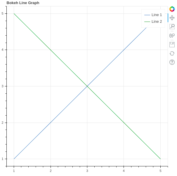
En el ejemplo anterior, hemos trazado dos líneas diferentes con una leyenda que simplemente indica cuál es la línea 1 y cuál es la línea 2. El color en las leyendas también se diferencia por el color.
Consulte los siguientes artículos para obtener información detallada sobre las anotaciones y leyendas.
Personalización de leyendas
Las leyendas en Bokeh se pueden personalizar usando las siguientes propiedades.
| Propiedad | Descripción |
|---|---|
| legend.label_text_font | cambiar la fuente de etiqueta predeterminada al nombre de fuente especificado |
| leyenda.etiqueta_texto_tamaño_fuente | tamaño de fuente en puntos |
| leyenda.ubicación | coloque la etiqueta en la ubicación especificada. |
| leyenda.título | establecer el título para la etiqueta de la leyenda |
| leyenda.orientación | establecer en horizontal (predeterminado) o vertical |
| legend.clicking_policy | especificar qué debe suceder cuando se hace clic en la leyenda |
Ejemplo:
Python3
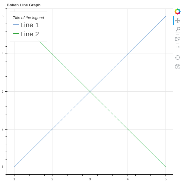
# importing the modules
from bokeh.plotting import figure, output_file, show

# instantiating the figure object
graph = figure(title="Bokeh Line Graph")

# the points to be plotted
x = [1, 2, 3, 4, 5]
y = [5, 4, 3, 2, 1]

# plotting the 1st line graph
graph.line(x, x, legend_label="Line 1")

# plotting the 2nd line graph with a
# different color
graph.line(y, x, legend_label="Line 2",
           line_color="green")

graph.legend.title = "Title of the legend"
graph.legend.location ="top_left"
graph.legend.label_text_font_size = "17pt"

# displaying the model
show(graph)
Producción:
Trazado de diferentes tipos de gráficos
Los glifos en la terminología de Bokeh se refieren a los componentes básicos de los diagramas de Bokeh, como líneas, rectángulos, cuadrados, etc. Los diagramas de Bokeh se crean mediante la interfaz bokeh.plotting , que utiliza un conjunto predeterminado de herramientas y estilos.
Gráfico de línea
Los gráficos de líneas se utilizan para representar la relación entre dos datos X e Y en un eje diferente. Se puede crear un diagrama de líneas utilizando el método line() del módulo de trazado.
Sintaxis:
línea (parámetros)
Ejemplo:
Python3
# importing the modules
from bokeh.plotting import figure, output_file, show

# instantiating the figure object
graph = figure(title = "Bokeh Line Graph")

# the points to be plotted
x = [1, 2, 3, 4, 5]
y = [5, 4, 3, 2, 1]

# plotting the line graph
graph.line(x, y)

# displaying the model
show(graph)
Producción:
Consulte los siguientes artículos para obtener información detallada sobre los diagramas de líneas.
Parcela de barra
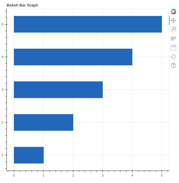
Diagrama de barras o gráfico de barras es un gráfico que representa la categoría de datos con barras rectangulares con longitudes y alturas proporcionales a los valores que representan. Puede ser de dos tipos barras horizontales y barras verticales. Cada uno se puede crear utilizando las funciones hbar() y vbar() de la interfaz de trazado, respectivamente.
Sintaxis:
hbar(parámetros)
vbar(parámetros)
Ejemplo 1: Creación de barras horizontales.
Python3
# importing the modules
from bokeh.plotting import figure, output_file, show

# instantiating the figure object
graph = figure(title = "Bokeh Bar Graph")

# the points to be plotted
x = [1, 2, 3, 4, 5]
y = [1, 2, 3, 4, 5]

# height / thickness of the plot
height = 0.5

# plotting the bar graph
graph.hbar(x, right = y, height = height)

# displaying the model
show(graph)
Producción:
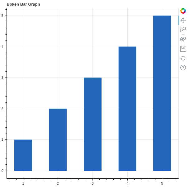
Ejemplo 2: Crear las barras verticales
Python3
# importing the modules
from bokeh.plotting import figure, output_file, show

# instantiating the figure object
graph = figure(title = "Bokeh Bar Graph")

# the points to be plotted
x = [1, 2, 3, 4, 5]
y = [1, 2, 3, 4, 5]

# height / thickness of the plot
width = 0.5

# plotting the bar graph
graph.vbar(x, top = y, width = width)

# displaying the model
show(graph)
Producción:
Consulte los siguientes artículos para obtener información detallada sobre los gráficos de barras.
- Python Bokeh: trazado de gráficos de barras horizontales
- Python Bokeh: trazado de gráficos de barras verticales
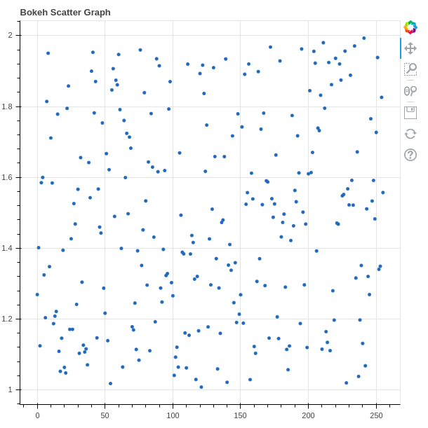
Gráfico de dispersión
Un gráfico de dispersión es un conjunto de puntos punteados para representar datos individuales en el eje horizontal y vertical. Un gráfico en el que los valores de dos variables se trazan a lo largo del eje X y el eje Y, el patrón de los puntos resultantes revela una correlación entre ellos. Se puede trazar utilizando el método scatter() del módulo de trazado.
Sintaxis:
scatter(parameters)
Ejemplo:
Python3
# importing the modules
from bokeh.plotting import figure, output_file, show
from bokeh.palettes import magma
import random


# instantiating the figure object
graph = figure(title = "Bokeh Scatter Graph")

# points to be plotted
x = [n for n in range(256)]
y = [random.random() + 1 for n in range(256)]


# plotting the graph
graph.scatter(x, y)

# displaying the model
show(graph)
Producción:
Consulte los artículos a continuación para obtener información detallada sobre los diagramas de dispersión.
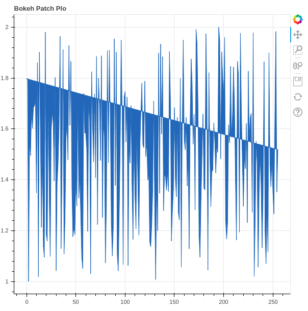
Gráfico de parche
Patch Plot sombrea una región del área para mostrar un grupo que tiene las mismas propiedades. Se puede crear utilizando el método patch() del módulo de trazado.
Sintaxis:
parche (parámetros)
Ejemplo:
Python3
# importing the modules
from bokeh.plotting import figure, output_file, show
from bokeh.palettes import magma
import random


# instantiating the figure object
graph = figure(title = "Bokeh Patch Plo")

# points to be plotted
x = [n for n in range(256)]
y = [random.random() + 1 for n in range(256)]

# plotting the graph
graph.patch(x, y)

# displaying the model
show(graph)
Producción:
Consulte los artículos a continuación para obtener información detallada sobre el gráfico de parches.
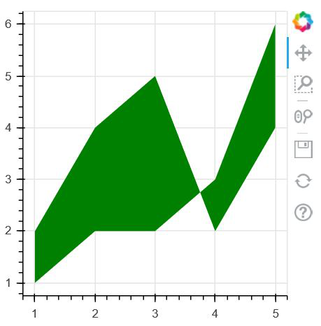
Parcela de área
Las parcelas de área se definen como las regiones rellenas entre dos series que comparten áreas comunes. La clase Bokeh Figure tiene dos métodos que son: varea(), harea()
Sintaxis:
varea(x, y1, y2, **kwargs)
harea(x1, x2, y, **kwargs)
Ejemplo 1: Creación de un gráfico de área vertical
Python
# Implementation of bokeh function
import numpy as np
from bokeh.plotting import figure, output_file, show

x = [1, 2, 3, 4, 5]
y1 = [2, 4, 5, 2, 4]
y2 = [1, 2, 2, 3, 6]

p = figure(plot_width=300, plot_height=300)

# area plot
p.varea(x=x, y1=y1, y2=y2,fill_color="green")

show(p)
Producción:
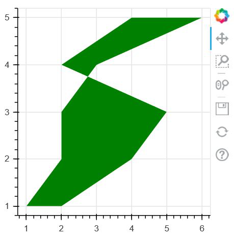
Ejemplo 2: Creación de un gráfico de área horizontal
Python3
# Implementation of bokeh function

import numpy as np
from bokeh.plotting import figure, output_file, show

y = [1, 2, 3, 4, 5]
x1 = [2, 4, 5, 2, 4]
x2 = [1, 2, 2, 3, 6]

p = figure(plot_width=300, plot_height=300)

# area plot
p.harea(x1=x1, x2=x2, y=y,fill_color="green")

show(p)
Producción:
Consulte los siguientes artículos para obtener información detallada sobre los gráficos de área
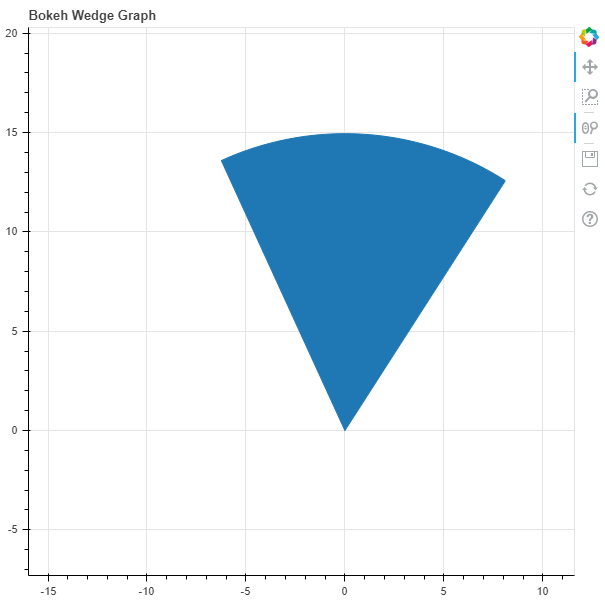
Gráfico circular
Bokeh No proporciona un método directo para trazar el gráfico circular. Se puede crear usando el método wedge() . En la función wedge(), los parámetros principales son las coordenadas x e y de la cuña, el radio, el start_angle y el end_angle de la cuña. Para trazar las cuñas de tal manera que se vean como un gráfico circular, los parámetros x, y y radio de todas las cuñas serán los mismos. Solo ajustaremos start_angle y end_angle.
Sintaxis:
cuña (parámetros)
Ejemplo:
Python3
# importing the modules
from bokeh.plotting import figure, output_file, show

# instantiating the figure object
graph = figure(title = "Bokeh Wedge Graph")

# the points to be plotted
x = 0
y = 0

# radius of the wedge
radius = 15

# start angle of the wedge
start_angle = 1

# end angle of the wedge
end_angle = 2

# plotting the graph
graph.wedge(x, y, radius = radius,
            start_angle = start_angle,
            end_angle = end_angle)

# displaying the model
show(graph)
Producción:
Consulte los siguientes artículos para obtener información detallada sobre los gráficos circulares.
Creando diferentes formas
La clase Figura en Bokeh nos permite crear glifos vectorizados de diferentes formas como círculo, rectángulo, óvalo, polígono, etc. Discutámoslos en detalle.
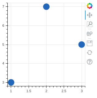
Circulo
La clase Bokeh Figure sigue los métodos para dibujar glifos circulares que se detallan a continuación:
- El método circle() se usa para agregar un glifo circular a la figura y necesita las coordenadas x e y de su centro.
- El método circle_cross() se usa para agregar un glifo circular con una cruz ‘+’ en el centro de la figura y necesita las coordenadas x e y de su centro.
- El método circle_x() se usa para agregar un glifo circular con una cruz ‘X’ en el centro. a la figura y necesita las coordenadas x e y de su centro.
Ejemplo:
Python3
import numpy as np
from bokeh.plotting import figure, output_file, show

# creating the figure object
plot = figure(plot_width = 300, plot_height = 300)

plot.circle(x = [1, 2, 3], y = [3, 7, 5], size = 20)

show(plot)
Producción:
Consulte los siguientes artículos para obtener información detallada sobre los glifos circulares.
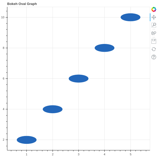
Oval
El método oval() se puede usar para trazar óvalos en el gráfico.
Sintaxis:
óvalo (parámetros)
Ejemplo:
Python3
# importing the modules
from bokeh.plotting import figure, output_file, show


# instantiating the figure object
graph = figure(title = "Bokeh Oval Graph")

# the points to be plotted
x = [1, 2, 3, 4, 5]
y = [i * 2 for i in x]

# plotting the graph
graph.oval(x, y,
        height = 0.5,
        width = 1)

# displaying the model
show(graph)
Producción:
Consulte los siguientes artículos para obtener información detallada sobre los glifos ovalados.
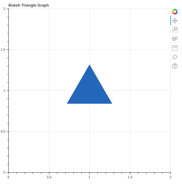
Triángulo
El triángulo se puede crear utilizando el método Triangle () .
Sintaxis:
triángulo (parámetros)
Ejemplo:
Python3
# importing the modules
from bokeh.plotting import figure, output_file, show


# instantiating the figure object
graph = figure(title = "Bokeh Triangle Graph")

# the points to be plotted
x = 1
y = 1

# plotting the graph
graph.triangle(x, y, size = 150)

# displaying the model
show(graph)
Producción:
Consulte el siguiente artículo para obtener información detallada sobre los triángulos.
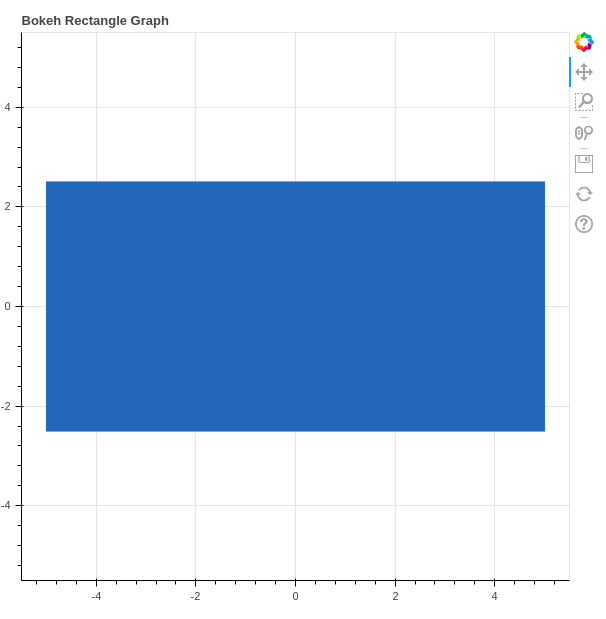
Rectángulo
Al igual que los círculos y los óvalos, el rectángulo también se puede trazar en Bokeh. Se puede trazar utilizando el método rect() .
Sintaxis:
rect(parámetros)
Ejemplo:
Python3
# importing the modules
from bokeh.plotting import figure, output_file, show


# instantiating the figure object
graph = figure(title = "Bokeh Rectangle Graph", match_aspect = True)

# the points to be plotted
x = 0
y = 0
width = 10
height = 5

# plotting the graph
graph.rect(x, y, width, height)

# displaying the model
show(graph)
Producción:
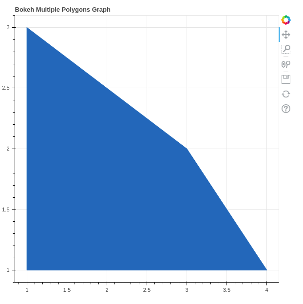
Polígono
Bokeh también se puede utilizar para trazar varios polígonos en un gráfico. El trazado de varios polígonos en un gráfico se puede realizar mediante el método multi_polygons() del módulo de trazado.
Sintaxis:
multi_polygons(parámetros)
Ejemplo:
Python3
# importing the modules
from bokeh.plotting import figure, output_file, show


# instantiating the figure object
graph = figure(title = "Bokeh Multiple Polygons Graph")

# the points to be plotted
xs = [[[[1, 1, 3, 4]]]]
ys = [[[[1, 3, 2 ,1]]]]

# plotting the graph
graph.multi_polygons(xs, ys)

# displaying the model
show(graph)
Producción:
Consulte los artículos a continuación para obtener información detallada sobre los glifos de polígono.
Trazado de múltiples parcelas
Hay varios diseños proporcionados por el Bokeh para crear Parcelas Múltiples. Estos diseños son:
- Disposición Vertical
- Disposición Horizontal
- Diseño de cuadrícula
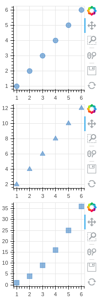
Diseños verticales
El diseño vertical establece todas las parcelas en forma vertical y se puede crear utilizando el método column() .
Python3
from bokeh.io import output_file, show
from bokeh.layouts import column
from bokeh.plotting import figure


x = [1, 2, 3, 4, 5, 6]
y0 = x
y1 = [i * 2 for i in x]
y2 = [i ** 2 for i in x]

# create a new plot
s1 = figure(width=200, plot_height=200)
s1.circle(x, y0, size=10, alpha=0.5)

# create another one
s2 = figure(width=200, height=200)
s2.triangle(x, y1, size=10, alpha=0.5)

# create and another
s3 = figure(width=200, height=200)
s3.square(x, y2, size=10, alpha=0.5)

# put all the plots in a VBox
p = column(s1, s2, s3)

# show the results
show(p)
Producción:
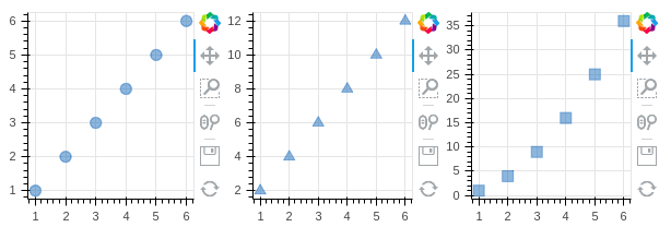
Disposición Horizontal
Diseño horizontal establece todas las parcelas en forma horizontal. Se puede crear usando el método row() .
Ejemplo:
Python3
from bokeh.io import output_file, show
from bokeh.layouts import row
from bokeh.plotting import figure


x = [1, 2, 3, 4, 5, 6]
y0 = x
y1 = [i * 2 for i in x]
y2 = [i ** 2 for i in x]

# create a new plot
s1 = figure(width=200, plot_height=200)
s1.circle(x, y0, size=10, alpha=0.5)

# create another one
s2 = figure(width=200, height=200)
s2.triangle(x, y1, size=10, alpha=0.5)

# create and another
s3 = figure(width=200, height=200)
s3.square(x, y2, size=10, alpha=0.5)

# put all the plots in a VBox
p = row(s1, s2, s3)

# show the results
show(p)
Producción:
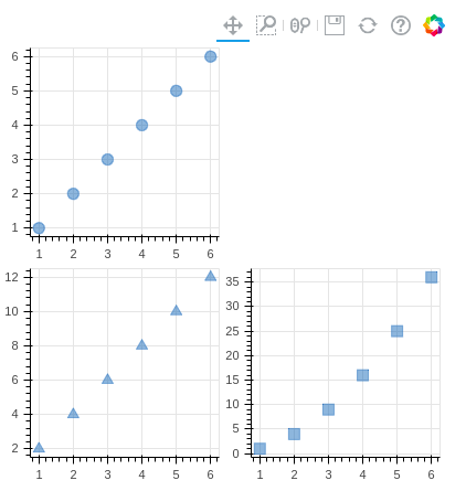
Diseño de cuadrícula
El método gridplot() se puede utilizar para organizar todos los gráficos en forma de cuadrícula. también podemos pasar Ninguno para dejar un espacio vacío para una trama.
Ejemplo:
Python3
from bokeh.io import output_file, show
from bokeh.layouts import gridplot
from bokeh.plotting import figure


x = [1, 2, 3, 4, 5, 6]
y0 = x
y1 = [i * 2 for i in x]
y2 = [i ** 2 for i in x]

# create a new plot
s1 = figure()
s1.circle(x, y0, size=10, alpha=0.5)

# create another one
s2 = figure()
s2.triangle(x, y1, size=10, alpha=0.5)

# create and another
s3 = figure()
s3.square(x, y2, size=10, alpha=0.5)

# put all the plots in a grid
p = gridplot([[s1, None], [s2, s3]], plot_width=200, plot_height=200)

# show the results
show(p)
Producción:
Visualización interactiva de datos
Una de las características clave de Bokeh que lo diferencia de otras bibliotecas de visualización es agregar interacción a la trama. Veamos varias interacciones que se pueden agregar a la trama.
Configuración de herramientas de trazado
En todos los gráficos anteriores, debe haber notado una barra de herramientas que aparece principalmente a la derecha del gráfico. Bokeh nos proporciona los métodos para manejar estas herramientas. Las herramientas se pueden clasificar en cuatro categorías.
- Gestos: estas herramientas manejan los gestos, como el movimiento panorámico. Hay tres tipos de gestos:
- Herramientas de movimiento panorámico/arrastre
- Herramientas de clic/toque
- Herramientas de desplazamiento/pellizco
- Acciones: estas herramientas manejan cuando se presiona un botón.
- Inspectores: estas herramientas informan o anotan el gráfico, como HoverTool.
- Herramientas de edición: estas son herramientas de gestos múltiples que pueden agregar, eliminar glifos del gráfico.
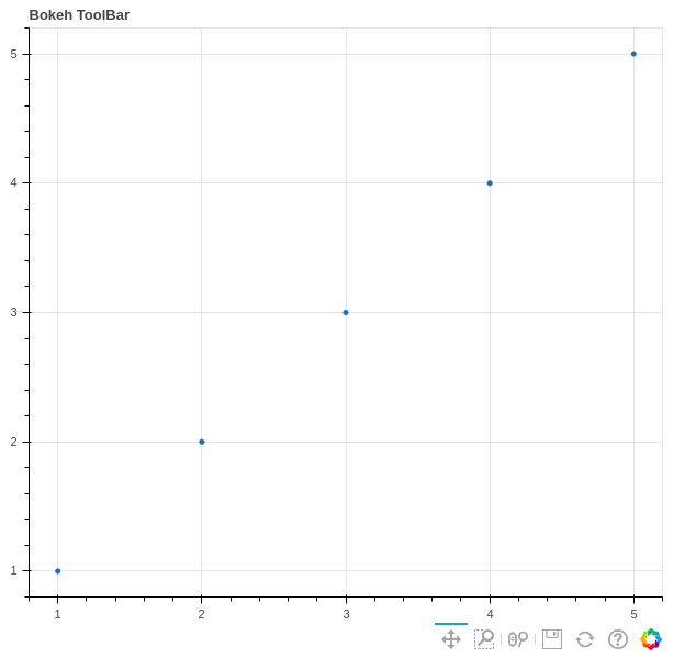
Ajuste de la posición de la barra de herramientas
Podemos especificar la posición de la barra de herramientas según nuestras propias necesidades. Se puede hacer pasando el parámetro toolbar_location al método figure() . El posible valor de este parámetro es:
- «arriba»
- «abajo»
- «izquierda»
- «Correcto»
Ejemplo:
Python3
# importing the modules
from bokeh.plotting import figure, output_file, show

# instantiating the figure object
graph = figure(title = "Bokeh ToolBar", toolbar_location="below")

# the points to be plotted
x = [1, 2, 3, 4, 5]
y = [1, 2, 3, 4, 5]

# height / thickness of the plot
width = 0.5

# plotting the scatter graph
graph.scatter(x, y)

# displaying the model
show(graph)
Producción:
Leyendas interactivas
En la sección de anotaciones y leyendas hemos visto la lista de todos los parámetros de las leyendas, sin embargo, aún no hemos discutido el parámetro click_policy . Esta propiedad hace que la leyenda sea interactiva. Hay dos tipos de interactividad:
- Ocultar: Oculta los Glifos.
- Silenciar: Ocultar el glifo hace que desaparezca por completo, por otro lado, silenciar el glifo simplemente quita énfasis al glifo en función de los parámetros.
Ejemplo 1: ocultar la leyenda
Python3
# importing the modules
from bokeh.plotting import figure, output_file, show

# file to save the model
output_file("gfg.html")

# instantiating the figure object
graph = figure(title = "Bokeh Hiding Glyphs")

# plotting the graph
graph.vbar(x = 1, top = 5,
        width = 1, color = "violet",
        legend_label = "Violet Bar")
graph.vbar(x = 2, top = 5,
        width = 1, color = "green",
        legend_label = "Green Bar")
graph.vbar(x = 3, top = 5,
        width = 1, color = "yellow",
        legend_label = "Yellow Bar")
graph.vbar(x = 4, top = 5,
        width = 1, color = "red",
        legend_label = "Red Bar")

# enable hiding of the glyphs
graph.legend.click_policy = "hide"

# displaying the model
show(graph)
Producción:
Ejemplo 2: silenciar la leyenda
Python3
# importing the modules
from bokeh.plotting import figure, output_file, show

# file to save the model
output_file("gfg.html")

# instantiating the figure object
graph = figure(title = "Bokeh Hiding Glyphs")

# plotting the graph
graph.vbar(x = 1, top = 5,
        width = 1, color = "violet",
        legend_label = "Violet Bar",
        muted_alpha=0.2)
graph.vbar(x = 2, top = 5,
        width = 1, color = "green",
        legend_label = "Green Bar",
        muted_alpha=0.2)
graph.vbar(x = 3, top = 5,
        width = 1, color = "yellow",
        legend_label = "Yellow Bar",
        muted_alpha=0.2)
graph.vbar(x = 4, top = 5,
        width = 1, color = "red",
        legend_label = "Red Bar",
        muted_alpha=0.2)

# enable hiding of the glyphs
graph.legend.click_policy = "mute"

# displaying the model
show(graph)
Producción:
Agregar widgets a la trama
Bokeh proporciona características de GUI similares a los formularios HTML como botones, control deslizante, casilla de verificación, etc. Estos proporcionan una interfaz interactiva para el gráfico que permite cambiar los parámetros del gráfico, modificar los datos del gráfico, etc. Veamos cómo usar y agregar algunos aparatos usados.
- Botones: este widget agrega un widget de botón simple al gráfico. Tenemos que pasar una función de JavaScript personalizada al método CustomJS() de la clase de modelos.
Sintaxis:
Botón (etiqueta, icono, devolución de llamada)
Ejemplo:
Python3
from bokeh.io import show
from bokeh.models import Button, CustomJS

button = Button(label="GFG")
button.js_on_click(CustomJS(
  code="console.log('button: click!', this.toString())"))

show(button)
Producción:

- CheckboxGroup: agrega una casilla de verificación estándar al gráfico. De manera similar a los botones, tenemos que pasar la función JavaScript personalizada al método CustomJS() de la clase de modelos.
Ejemplo:
Python3
from bokeh.io import show
from bokeh.models import CheckboxGroup, CustomJS

L = ["First", "Second", "Third"]

# the active parameter sets checks the selected value
# by default
checkbox_group = CheckboxGroup(labels=L, active=[0, 2])

checkbox_group.js_on_click(CustomJS(code="""
    console.log('checkbox_group: active=' + this.active, this.toString())
"""))

show(checkbox_group)
Producción:

- RadioGroup: agrega un botón de radio simple y acepta una función de JavaScript personalizada.
Sintaxis:
RadioGroup(etiquetas, activo)
Ejemplo:
Python3
from bokeh.io import show
from bokeh.models import RadioGroup, CustomJS

L = ["First", "Second", "Third"]

# the active parameter sets checks the selected value
# by default
radio_group = RadioGroup(labels=L, active=1)

radio_group.js_on_click(CustomJS(code="""
    console.log('radio_group: active=' + this.active, this.toString())
"""))

show(radio_group)
Producción:

- Controles deslizantes: agrega un control deslizante al gráfico. También necesita una función JavaScript personalizada.
Sintaxis:
Control deslizante (inicio, fin, paso, valor)
Ejemplo:
Python3
from bokeh.io import show
from bokeh.models import CustomJS, Slider

slider = Slider(start=1, end=20, value=1, step=2, title="Slider")

slider.js_on_change("value", CustomJS(code="""
    console.log('slider: value=' + this.value, this.toString())
"""))

show(slider)
Producción:
- DropDown: agrega un menú desplegable a la trama y, como cualquier otro widget, también necesita una función de JavaScript personalizada como devolución de llamada.
Ejemplo:
Python3
from bokeh.io import show
from bokeh.models import CustomJS, Dropdown

menu = [("First", "First"), ("Second", "Second"), ("Third", "Third")]

dropdown = Dropdown(label="Dropdown Menu", button_type="success", menu=menu)

dropdown.js_on_event("menu_item_click", CustomJS(
    code="console.log('dropdown: ' + this.item, this.toString())"))

show(dropdown)
Producción:
- Widget de pestañas : Widget de pestañas agrega pestañas y cada pestaña muestra un gráfico diferente.
Ejemplo:
Python3
from bokeh.plotting import figure, output_file, show
from bokeh.models import Panel, Tabs
import numpy as np
import math


fig1 = figure(plot_width=300, plot_height=300)

x = [1, 2, 3, 4, 5]
y = [5, 4, 3, 2, 1]

fig1.line(x, y, line_color='green')
tab1 = Panel(child=fig1, title="Tab 1")

fig2 = figure(plot_width=300, plot_height=300)

fig2.line(y, x, line_color='red')
tab2 = Panel(child=fig2, title="Tab 2")

all_tabs = Tabs(tabs=[tab1, tab2])

show(all_tabs)
Producción:
Crear diferentes tipos de glifos
- Glifo de diamante
- Glifo de guión
- Cruz Glifo
- Glifo de diamante
- Glifo de cruz de diamante
- Glifo de punto de diamante
- Glifo de rayos
- Glifo de alfileres triangulares
- Triángulo con glifo de puntos
- Glifo de triángulo invertido
- Glifo más
- Glifo Cuadrilátero
- Glifo Y
- Glifo X
- Glifo ovalado
- Glifo hexagonal
- Glifo de mosaicos hexagonales
- Glifo de puntos hexagonales
- Cuadrado con Glifo de Cruz
- Cuadrado con glifo de puntos
- Cuadrado con Glifo de X
- Glifo de elipse
- Glifo de anillo
- Glifo de Bézier
- Glifo de asterisco
- Glifo de cuña anular
- Glifo de paso
Visualización de diferentes tipos de datos
- Python Bokeh: visualización del conjunto de datos de Iris
- Python Bokeh: visualización de datos de stock
- Visualización interactiva de datos usando Bokeh
Más temas sobre Bokeh
- Python Bokeh – Clase de colores
- ¿Cómo usar paletas de colores en Python-Bokeh?
- Python Bokeh: trazado de curvas cuadráticas en un gráfico
- Python Bokeh: trazado de segmentos de línea en un gráfico
- Python Bokeh: trazado de varias líneas en un gráfico
- Python Bokeh: trazado de glifos en un mapa de Google
- Python Bokeh: trazado para todos los tipos de Google Maps (hoja de ruta, satélite, híbrido, terreno)
Publicación traducida automáticamente
Artículo escrito por GeeksforGeeks-1 y traducido por Barcelona Geeks. The original can be accessed here. Licence: CCBY-SA