Comprender la regresión logística

Requisito previo: regresión lineal 
Este artículo analiza los conceptos básicos de la regresión logística y su implementación en Python. La regresión logística es básicamente un algoritmo de clasificación supervisado. En un problema de clasificación, la variable objetivo (o salida), y, solo puede tomar valores discretos para un conjunto dado de características (o entradas), X.
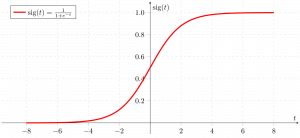
Contrariamente a la creencia popular, la regresión logística ES un modelo de regresión. El modelo construye un modelo de regresión para predecir la probabilidad de que una determinada entrada de datos pertenezca a la categoría numerada como «1». Al igual que la regresión lineal asume que los datos siguen una función lineal, la regresión logística modela los datos utilizando la función sigmoidea.

 

import csv
import numpy as np
import matplotlib.pyplot as plt
  
  
def loadCSV(filename):
    '''
    function to load dataset
    '''
    with open(filename,"r") as csvfile:
        lines = csv.reader(csvfile)
        dataset = list(lines)
        for i in range(len(dataset)):
            dataset[i] = [float(x) for x in dataset[i]]     
    return np.array(dataset)
  
  
def normalize(X):
    '''
    function to normalize feature matrix, X
    '''
    mins = np.min(X, axis = 0)
    maxs = np.max(X, axis = 0)
    rng = maxs - mins
    norm_X = 1 - ((maxs - X)/rng)
    return norm_X
  
  
def logistic_func(beta, X):
    '''
    logistic(sigmoid) function
    '''
    return 1.0/(1 + np.exp(-np.dot(X, beta.T)))
  
  
def log_gradient(beta, X, y):
    '''
    logistic gradient function
    '''
    first_calc = logistic_func(beta, X) - y.reshape(X.shape[0], -1)
    final_calc = np.dot(first_calc.T, X)
    return final_calc
  
  
def cost_func(beta, X, y):
    '''
    cost function, J
    '''
    log_func_v = logistic_func(beta, X)
    y = np.squeeze(y)
    step1 = y * np.log(log_func_v)
    step2 = (1 - y) * np.log(1 - log_func_v)
    final = -step1 - step2
    return np.mean(final)
  
  
def grad_desc(X, y, beta, lr=.01, converge_change=.001):
    '''
    gradient descent function
    '''
    cost = cost_func(beta, X, y)
    change_cost = 1
    num_iter = 1
      
    while(change_cost > converge_change):
        old_cost = cost
        beta = beta - (lr * log_gradient(beta, X, y))
        cost = cost_func(beta, X, y)
        change_cost = old_cost - cost
        num_iter += 1
      
    return beta, num_iter 
  
  
def pred_values(beta, X):
    '''
    function to predict labels
    '''
    pred_prob = logistic_func(beta, X)
    pred_value = np.where(pred_prob >= .5, 1, 0)
    return np.squeeze(pred_value)
  
  
def plot_reg(X, y, beta):
    '''
    function to plot decision boundary
    '''
    # labelled observations
    x_0 = X[np.where(y == 0.0)]
    x_1 = X[np.where(y == 1.0)]
      
    # plotting points with diff color for diff label
    plt.scatter([x_0[:, 1]], [x_0[:, 2]], c='b', label='y = 0')
    plt.scatter([x_1[:, 1]], [x_1[:, 2]], c='r', label='y = 1')
      
    # plotting decision boundary
    x1 = np.arange(0, 1, 0.1)
    x2 = -(beta[0,0] + beta[0,1]*x1)/beta[0,2]
    plt.plot(x1, x2, c='k', label='reg line')
  
    plt.xlabel('x1')
    plt.ylabel('x2')
    plt.legend()
    plt.show()
      
  
      
if __name__ == "__main__":
    # load the dataset
    dataset = loadCSV('dataset1.csv')
      
    # normalizing feature matrix
    X = normalize(dataset[:, :-1])
      
    # stacking columns with all ones in feature matrix
    X = np.hstack((np.matrix(np.ones(X.shape[0])).T, X))
  
    # response vector
    y = dataset[:, -1]
  
    # initial beta values
    beta = np.matrix(np.zeros(X.shape[1]))
  
    # beta values after running gradient descent
    beta, num_iter = grad_desc(X, y, beta)
  
    # estimated beta values and number of iterations
    print("Estimated regression coefficients:", beta)
    print("No. of iterations:", num_iter)
  
    # predicted labels
    y_pred = pred_values(beta, X)
      
    # number of correctly predicted labels
    print("Correctly predicted labels:", np.sum(y == y_pred))
      
    # plotting regression line
    plot_reg(X, y, beta)

from sklearn import datasets, linear_model, metrics
   
# load the digit dataset
digits = datasets.load_digits()
   
# defining feature matrix(X) and response vector(y)
X = digits.data
y = digits.target
  
# splitting X and y into training and testing sets
from sklearn.model_selection import train_test_split
X_train, X_test, y_train, y_test = train_test_split(X, y, test_size=0.4,
                                                    random_state=1)
   
# create logistic regression object
reg = linear_model.LogisticRegression()
   
# train the model using the training sets
reg.fit(X_train, y_train)
  
# making predictions on the testing set
y_pred = reg.predict(X_test)
   
# comparing actual response values (y_test) with predicted response values (y_pred)
print("Logistic Regression model accuracy(in %):", 
metrics.accuracy_score(y_test, y_pred)*100)