Gráfica de amplitud y fase de demodulación compleja

Gráfica de fase de demodulación compleja

En el análisis de frecuencia de modelos de series de tiempo, un modelo común es una onda sinusoidal:

$Y_{i} = C + \alpha\sin{(2\pi\omega t_{i} + \phi)} + E_{i}$

donde, ∝ es la amplitud, phi es el cambio de fase y omega es la frecuencia dominante. El objetivo de la gráfica de demodulación compleja es mejorar la estimación de frecuencia.

Las gráficas de demodulación complejas formadas por dos componentes:

Eje vertical: Fase
Eje horizontal: Tiempo

Importancia de una Buena Estimación Inicial de la Frecuencia:

El ajuste no lineal para las ondas sinusoidales

$Y_{i} = C + \alpha\sin{(2\pi\omega t_{i} + \phi)} + E_{i}$

La ecuación anterior es sensible a buenos valores iniciales. El valor inicial de la frecuencia omega se puede obtener mediante el gráfico espectral. El gráfico de fase de demodulación compleja se utiliza para evaluar si esta estimación es adecuada. Si la estimación no es adecuada, entonces si debe aumentarse o disminuirse.

Gráfica de amplitud de demodulación compleja:

En el análisis de frecuencia de modelos de series de tiempo, un modelo común es una onda sinusoidal:

$Y_{i} = C + \alpha\sin{(2\pi\omega t_{i} + \phi)} + E_{i}$

donde, ∝ es la amplitud, phi es el cambio de fase y omega es la frecuencia dominante.

Si la pendiente de la gráfica de amplitud de demodulación compleja no es cero, entonces la ecuación anterior finalmente se reemplaza por el modelo.

$Y_{i} = C + \alpha_{i}\sin{(2\pi\omega t_{i} + \phi)} + E_{i}$

donde, a _i es algún tipo de ajuste de modelo lineal con mínimos cuadrados estándar. El caso más común es el ajuste lineal, es decir, el modelo queda de la siguiente manera:

$Y_{i} = C + (B_0 + B_1*t_{i})\sin{(2\pi\omega t_{i} + \phi)} + E_{i}$

La gráfica de amplitud de demodulación compleja está formada por

Eje vertical: Amplitud
Eje horizontal: Tiempo

El gráfico de demodulación de amplitud compleja responde a las siguientes preguntas:

¿Cambia la amplitud con el tiempo?
¿Hay algún efecto de puesta en marcha que condujo a que la amplitud fuera inestable al principio?
¿Hay algún valor atípico en amplitud?

Implementación:
Código: código Python para análisis de demodulación compleja

python3

# code
import numpy as np
import matplotlib.pyplot as plt
 
def gen_test_data(periods, noise=0, rotary=False, npts=1000, dt=1.0/24):
    """
    Generate a simple time series for testing complex demodulation.
     
    *periods* is a sequence with the periods of one or more
        harmonics that will be added to make the test signal.
        They can be positive or negative.
    *noise* is the amplitude of independent Gaussian noise.   
    *rotary* is Boolean; if True, the test signal is complex.
    *npts* is the length of the series.
    *dt* is the time interval (default is 1.0/24)
     
    Returns t, x: ndarrays with the test times and test data values..
    """    
         
    t = np.arange(npts, dtype=float) * dt
     
    if rotary:
        x = noise * (np.random.randn(npts) + 1j * np.random.randn(npts))
    else:
        x = noise * np.random.randn(npts)
 
    for p in periods:
        if rotary:
            x += np.exp(2j * np.pi * t / p)
        else:
            x += np.cos(2 * np.pi * t / p)
     
    return t, x
   
def complex_demodulation(t, x, central_period, hwidth = 2):
    """
    Complex demodulation of a real or complex series, *x*
    of samples at times *t*, assumed to be uniformly spaced.
     
    *central_period* is the period of the central frequency
        for the demodulation.  It should be positive for real
        signals. For complex signals, a positive value will
        return the CCW rotary component, and a negative value
        will return the CW component (negative frequency).
        Period is in the same time units as are used for *t*.
 
    *hwidth* is the Blackman filter half-width in units of the
        *central_period*.  For example, the default value of 2
        makes the Blackman half-width equal to twice the
        central period.
     
    Returns a dictionary.
    """    
     
    rotary = x.dtype.kind == 'c'  # complex input
     
    # Make the complex exponential for demodulation:
    c = np.exp(-1j * 2 * np.pi * t / central_period)
     
    product = x * c
     
    # filter half-width number of points
    dt = t[1] - t[0]
    hwpts = int(round(hwidth * abs(central_period) / dt))
    nf = hwpts * 2 + 1
    x1 = np.linspace(-1, 1, nf, endpoint=True)
    x1 = x1[1:-1]   # chop off the useless endpoints with zero weight
    w1 = 0.42 + 0.5 * np.cos(x1 * np.pi) + 0.08 * np.cos(x1 * 2 * np.pi)
    ytop = np.convolve(product, w1, mode='same')
    ybot = np.convolve(np.ones_like(product), w1, mode='same')
    demod = ytop/ybot
    if not rotary:   
        # The factor of 2 below comes from fact that the
        # mean value of a squared unit sinusoid is 0.5.
        demod *= 2
     
    reconstructed = (demod * np.conj(c))
    if not rotary:
        reconstructed = reconstructed.real
         
    if np.sign(central_period) < 0:
        demod = np.conj(demod)
        # This is to make the phase increase in time
        # for both positive and negative demod frequency
        # when the frequency of the signal exceeds the
        # frequency of the demodulation.
     
    d = {'t':t,'signal' : x,'hwpts' : hwpts,'demod': demod,'reconstructed' : reconstructed}
    return d
   
def plot_demodulation(dm):
    fig, axs = plt.subplots(3, sharex=True)
    resid = dm.get('signal') - dm.get('reconstructed')
    if dm.get('signal').dtype.kind == 'c':
        axs[0].plot(dm.get('t'), dm.get('signal').real, label='signal.real')
        axs[0].plot(dm.get('t'), dm.get('signal').imag, label='signal.imag')
        axs[0].plot(dm.get('t'), resid.real, label='difference real')
        axs[0].plot(dm.get('t'), resid.imag, label='difference imag')
    else:   
        axs[0].plot(dm.get('t'), dm.get('signal'), label='signal')
        axs[0].plot(dm.get('t'), dm.get('reconstructed'), label='reconstructed')
        axs[0].plot(dm.get('t'), dm.get('signal') - dm.get('reconstructed'), label='difference')
     
    axs[0].legend(loc='upper right', fontsize='small')
     
    axs[1].plot(dm.get('t'), np.abs(dm.get('demod')), label='amplitude', color='C3')
    axs[1].legend(loc='upper right', fontsize='small')
     
    axs[2].plot(dm.get('t'), np.angle(dm.get('demod'), deg=True), '.', label='phase',
                color='C4')
    axs[2].set_ylim(-180, 180)
    axs[2].legend(loc='upper right', fontsize='small')
     
    for ax in axs:
        ax.locator_params(axis='y', nbins=5)
    return fig, axs
 
def test_demodulation(periods, central_period,
                 noise=0,
                 rotary=False,
                 hwidth = 1,
                 npts=1000,
                 dt=1.0/24):
     
    t, x = gen_test_data(periods, noise=noise, rotary=rotary,
                     npts=npts, dt=dt)
    dm = complex_demodulation(t, x, central_period, hwidth=hwidth)
    fig, axs = plot_demodulation(dm)
    return fig, axs, dm
# Example 1
test_demodulation([12.0/24], 12.0/24);
# Example 2
test_demodulation([11.0/24], 12.0/24)

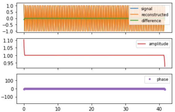
Ejemplo 1: señal, demodulación de amplitud y demodulación de fase

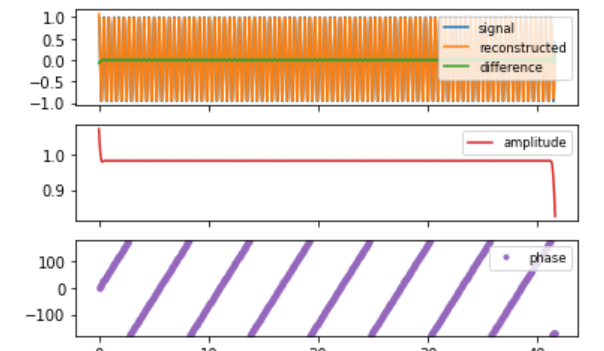
Ejemplo 2: señal, demodulación de amplitud y demodulación de fase

Publicación traducida automáticamente

Artículo escrito por pawangfg y traducido por Barcelona Geeks. The original can be accessed here. Licence: CCBY-SA

Gráfica de fase de demodulación compleja

Importancia de una Buena Estimación Inicial de la Frecuencia:

Gráfica de amplitud de demodulación compleja:

Implementación: Código: código Python para análisis de demodulación compleja

python3

Deja una respuesta Cancelar la respuesta

Implementación:
Código: código Python para análisis de demodulación compleja