Implementación de Agglomerative Clustering usando Sklearn

Requisitos previos: Agglomerative Clustering Agglomerative Clustering es una de las técnicas de agrupación jerárquica más comunes. Conjunto de datos: conjunto de datos de tarjetas de crédito . Suposición: la técnica de agrupamiento asume que cada punto de datos es lo suficientemente similar a los otros puntos de datos que se puede suponer que los datos al principio están agrupados en 1 grupo. Paso 1: Importación de las bibliotecas requeridas 

import pandas as pd
import numpy as np
import matplotlib.pyplot as plt
from sklearn.decomposition import PCA
from sklearn.cluster import AgglomerativeClustering
from sklearn.preprocessing import StandardScaler, normalize
from sklearn.metrics import silhouette_score
import scipy.cluster.hierarchy as shc

Paso 2: Cargar y Limpiar los datos 

# Changing the working location to the location of the file
cd C:\Users\Dev\Desktop\Kaggle\Credit_Card
 
X = pd.read_csv('CC_GENERAL.csv')
 
# Dropping the CUST_ID column from the data
X = X.drop('CUST_ID', axis = 1)
 
# Handling the missing values
X.fillna(method ='ffill', inplace = True)

Paso 3: Preprocesamiento de los datos 

# Scaling the data so that all the features become comparable
scaler = StandardScaler()
X_scaled = scaler.fit_transform(X)
 
# Normalizing the data so that the data approximately
# follows a Gaussian distribution
X_normalized = normalize(X_scaled)
 
# Converting the numpy array into a pandas DataFrame
X_normalized = pd.DataFrame(X_normalized)

Paso 4: Reducir la dimensionalidad de los Datos 

pca = PCA(n_components = 2)
X_principal = pca.fit_transform(X_normalized)
X_principal = pd.DataFrame(X_principal)
X_principal.columns = ['P1', 'P2']

Los dendogramas se utilizan para dividir un grupo dado en muchos grupos diferentes. Paso 5: Visualización del funcionamiento de los Dendogramas 

plt.figure(figsize =(8, 8))
plt.title('Visualising the data')
Dendrogram = shc.dendrogram((shc.linkage(X_principal, method ='ward')))

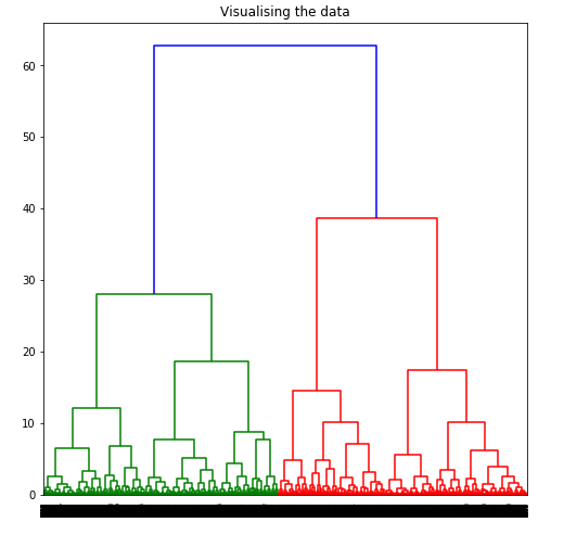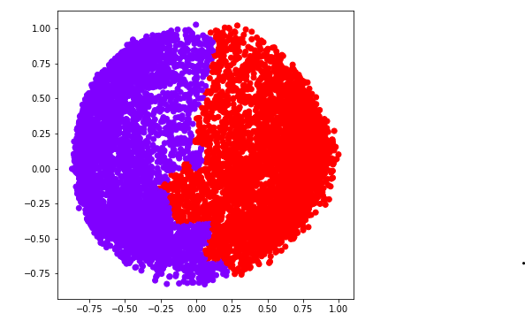
To determine the optimal number of clusters by visualizing the data, imagine all the horizontal lines as being completely horizontal and then after calculating the maximum distance between any two horizontal lines, draw a horizontal line in the maximum distance calculated. 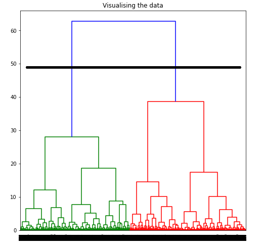The above image shows that the optimal number of clusters should be 2 for the given data. Step 6: Building and Visualizing the different clustering models for different values of k a) k = 2 

ac2 = AgglomerativeClustering(n_clusters = 2)
 
# Visualizing the clustering
plt.figure(figsize =(6, 6))
plt.scatter(X_principal['P1'], X_principal['P2'],
           c = ac2.fit_predict(X_principal), cmap ='rainbow')
plt.show()

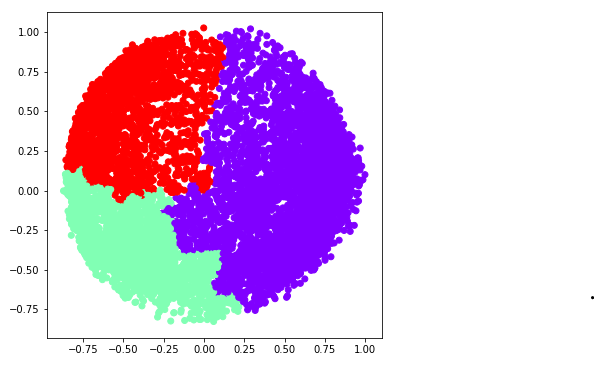
b) k = 3 

ac3 = AgglomerativeClustering(n_clusters = 3)
 
plt.figure(figsize =(6, 6))
plt.scatter(X_principal['P1'], X_principal['P2'],
           c = ac3.fit_predict(X_principal), cmap ='rainbow')
plt.show()

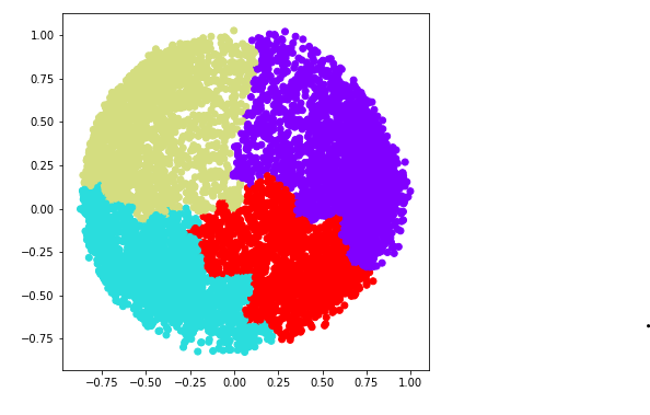
c) k = 4 

ac4 = AgglomerativeClustering(n_clusters = 4)
 
plt.figure(figsize =(6, 6))
plt.scatter(X_principal['P1'], X_principal['P2'],
            c = ac4.fit_predict(X_principal), cmap ='rainbow')
plt.show()

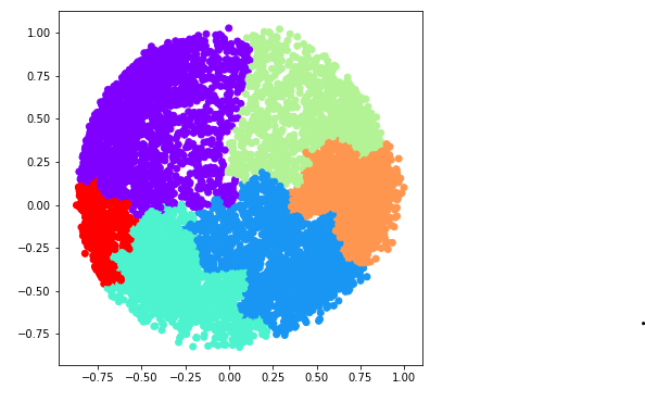
d) k = 5 

ac5 = AgglomerativeClustering(n_clusters = 5)
 
plt.figure(figsize =(6, 6))
plt.scatter(X_principal['P1'], X_principal['P2'],
            c = ac5.fit_predict(X_principal), cmap ='rainbow')
plt.show()

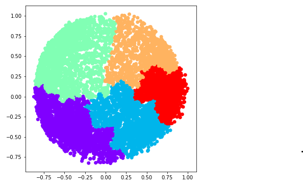e) k = 6 

ac6 = AgglomerativeClustering(n_clusters = 6)
 
plt.figure(figsize =(6, 6))
plt.scatter(X_principal['P1'], X_principal['P2'],
            c = ac6.fit_predict(X_principal), cmap ='rainbow')
plt.show()

We now determine the optimal number of clusters using a mathematical technique. Here, We will use the Silhouette Scores for the purpose. Step 7: Evaluating the different models and Visualizing the results. 

k = [2, 3, 4, 5, 6]
 
# Appending the silhouette scores of the different models to the list
silhouette_scores = []
silhouette_scores.append(
        silhouette_score(X_principal, ac2.fit_predict(X_principal)))
silhouette_scores.append(
        silhouette_score(X_principal, ac3.fit_predict(X_principal)))
silhouette_scores.append(
        silhouette_score(X_principal, ac4.fit_predict(X_principal)))
silhouette_scores.append(
        silhouette_score(X_principal, ac5.fit_predict(X_principal)))
silhouette_scores.append(
        silhouette_score(X_principal, ac6.fit_predict(X_principal)))
 
# Plotting a bar graph to compare the results
plt.bar(k, silhouette_scores)
plt.xlabel('Number of clusters', fontsize = 20)
plt.ylabel('S(i)', fontsize = 20)
plt.show()

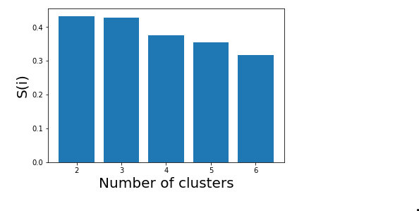Thus, with the help of the silhouette scores, it is concluded that the optimal number of clusters for the given data and clustering technique is 2.