TensorFlow, la plataforma de código abierto enormemente popular para desarrollar e integrar IA a gran escala y modelos de aprendizaje profundo, se actualizó recientemente a su nueva forma TensorFlow 2.0. Esto trae un impulso masivo en las funciones en el ecosistema ML originalmente rico en funciones creado por la comunidad TensorFlow.
¿Qué es el código abierto y cómo hizo que TensorFlow tuviera tanto éxito?
Código abierto significa algo que las personas (principalmente los desarrolladores) pueden modificar, compartir e integrar porque todas las características de diseño originales están abiertas para todos. Esto hace que sea muy fácil para un producto de software en particular expandirse de manera fácil, efectiva y en muy poco tiempo. Esta función permitió al creador original de TensorFlow, es decir, Google, trasladarlo fácilmente a todas las plataformas disponibles en el mercado, que incluye web, dispositivos móviles, Internet de las cosas, sistemas integrados, Edge Computing e incluye compatibilidad con varios otros lenguajes, como JavaScript, Node.js, F#, C++, C#, React.js, Go, Julia, Rust, Android, Swift, Kotlin y muchos otros.
Junto con esto, vino el soporte para la aceleración de hardware para ejecutar códigos de aprendizaje automático a gran escala. Estos incluyen CUDA (biblioteca para ejecutar código ML en GPU), TPU (Unidad de procesamiento de tensores: hardware personalizado proporcionado por Google especialmente diseñado y desarrollado para procesar tensores usando TensorFlow) para configuración de múltiples máquinas, GPU, GPGPU, TPU basados en la nube, ASIC ( Circuitos integrados específicos de la aplicación) FPGA (arrays de puertas programables en campo: se utilizan exclusivamente para hardware programable personalizado). Esto también incluye nuevas incorporaciones como los chips Jetson TX2 de NVIDIA y Movidius de Intel.
Ahora volviendo al TensorFlow2.0 más nuevo y rico en funciones:
esta es una implementación gráfica de los cambios:
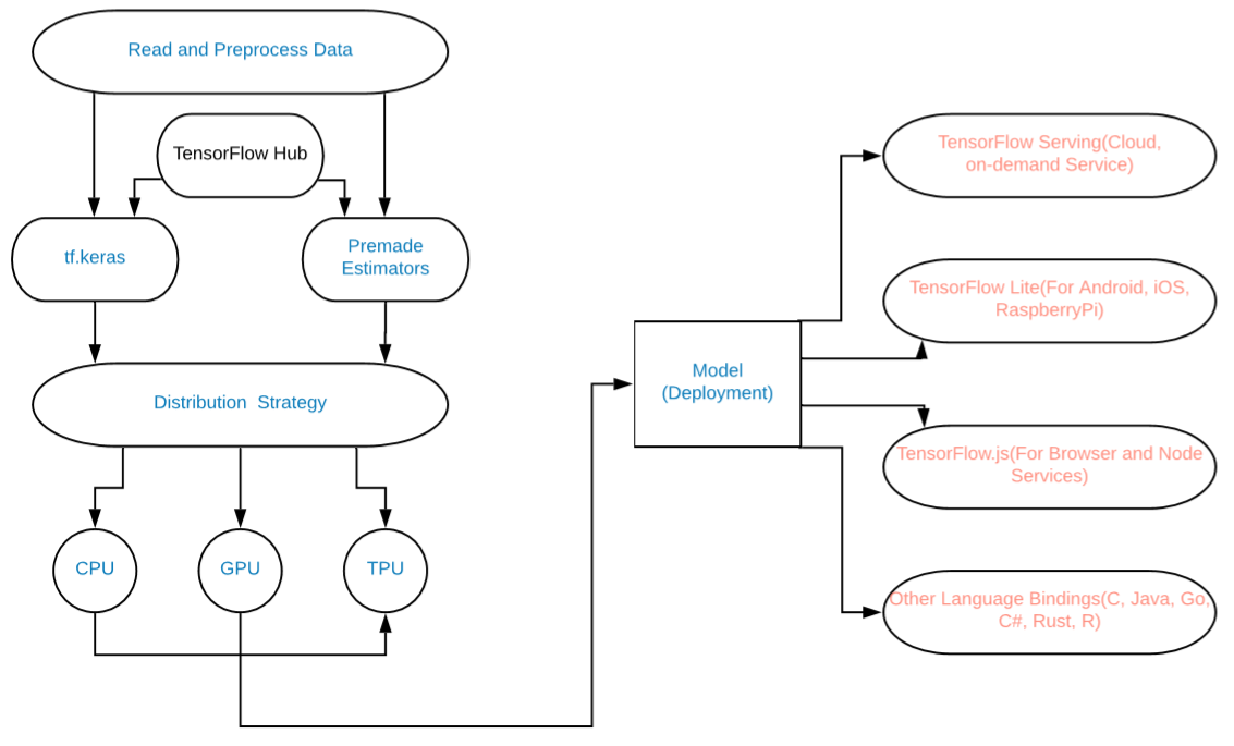
Diagrama del modelo
Las cosas que se agregan incluyen:
- Uso de tf.data para la carga de datos (o NumPy).
- Use Keras para la construcción de modelos. (También podemos usar cualquier Estimador prefabricado).
- Use tf.function para la ejecución de gráficos DAG o use una ejecución ansiosa.
- Utilice la estrategia de distribución para computación de alto rendimiento y modelos de aprendizaje profundo. (Para TPU, GPU, etc.).
- TF 2.0 estandariza el modelo guardado como una versión serializada de un gráfico TensorFlow para una variedad de plataformas diferentes que van desde Mobile, JavaScript, TensorBoard, TensorHub, etc.
Por fin, ahora podemos construir grandes modelos de ML y Deep Learning de manera fácil y efectiva en TensorFlow2.0 para usuarios finales e implementarlos a gran escala.
Ejemplos:
entrenamiento de una red neuronal para categorizar datos MNSIT
# Write Python3 code here
import tensorflow as tf

"""The Fashion MNIST data is available directly in the tf.keras
 datasets API. You load it like this:"""

mnist = tf.keras.datasets.fashion_mnist

"""Calling load_data on this object will give you two sets of two
 lists, these will be the training and testing values for the graphics
 that contain the clothing items and their labels."""

(training_images, training_labels), (test_images, test_labels) = mnist.load_data()
"""You'll notice that all of the values in the number are between 0 and 255.
If we are training a neural network, for various reasons it's easier if we
treat all values as between 0 and 1, a process called '**normalizing**'...and
fortunately in Python it's easy to normalize a list like this without looping.
So, perform it like - """

training_images  = training_images / 255.0
test_images = test_images / 255.0

"""Now you might be wondering why there are 2 sets...training and testing
-- remember we spoke about this in the intro? The idea is to have 1 set of
data for training, and then another set of data...that the model hasn't yet
seen...to see how good it would be at classifying values. After all, when
you're done, you're going to want to try it out with data that it hadn't
previously seen!

Let's now design the model. There are quite a few new concepts here,
but don't worry, you'll get the hang of them.
"""

model = tf.keras.models.Sequential([tf.keras.layers.Flatten(),
                                    tf.keras.layers.Dense(
                                            128, activation=tf.nn.relu),
                                    tf.keras.layers.Dense(
                                            10, activation=tf.nn.softmax)])

"""**Sequential**: That defines a SEQUENCE of layers in the neural network

**Flatten**: Remember earlier where our images were a square when
you printed them out? Flatten just takes that square and turns it
into a 1-dimensional set.

**Dense**: Adds a layer of neurons

Each layer of neurons needs an **activation function** to tell them what to
do. There are lots of options, but just use these for now.

**Relu** effectively means "If X>0 return X, else return 0" -- so what it does
 it only passes values 0 or greater to the next layer in the network.

**Softmax** takes a set of values, and effectively picks the biggest one, so,
 for example, if the output of the last layer looks like [0.1, 0.1, 0.05, 0.1,
 9.5, 0.1, 0.05, 0.05, 0.05], it saves you from fishing through it looking for
 the biggest value, and turns it into [0,0,0,0,1,0,0,0,0] --
 The goal is to save a lot of coding!

The next thing to do, now the model is defined, is to actually build it.
You do this by compiling it with an optimizer and loss function as before --
and then you train it by calling **model.fit ** asking it to fit your training
data to your training labels -- i.e. have it figure out the relationship between
the training data and its actual labels, so in future, if you have data that
looks like the training data, then it can make a prediction for what that data
would look like.
"""

model.compile(optimizer = tf.keras.optimizers.Adam(),
              loss = 'sparse_categorical_crossentropy',
              metrics=['accuracy'])

model.fit(training_images, training_labels, epochs=5)

"""Once it's done training -- you should see an accuracy value at the end of the
final epoch. It might look something like 0.9098. This tells you that your
neural network is about 91% accurate in classifying the training data. I.E.,
it figured out a pattern match between the image and the labels that worked
91% of the time. Not great, but not bad considering it was only trained for 5
epochs and done quite quickly.

But how would it work with unseen data? That's why we have the test images. We
can call model.evaluate, and pass in the two sets, and it will report back the
loss for each. Let's give it a try:
"""

model.evaluate(test_images, test_labels)

""" For me, that returned an accuracy of about .8838, which means it was
about 88% accurate. As expected it probably would not do as well with *unseen*
data as it did with data it was trained on!
 """
Producción:
Expected Accuracy 88-91%
Ejecución ansiosa:
import tensorflow as tf
import tensorflow.contrib.eager as tfe

tfe.enable_eager_execution()

x = [[2.]]
m = tf.matmul(x, x)

print(m)
Producción :
tf.Tensor([[4.]], shape=(1, 1), dtype=float32)
Publicación traducida automáticamente
Artículo escrito por hiteshsangwan0567 y traducido por Barcelona Geeks. The original can be accessed here. Licence: CCBY-SA